Random tips on working with the MLIR (LLVM) (and, possibly, other large C++ codebases). These are in no particular order¹. Skim (don’t peruse) and come back and use ctrl+f.

I’m going to walk through how to port PyTorch model (OPT) to MLIR, starting from the :hug: Hugging Face (HF) implementation.

Setting

Suppose you have this MLIR program representing two nested for loops:

// loops.mlir

#map0 = affine_map<(d0, d1) -> (d0)>
#map1 = affine_map<(d0, d1) -> (d1)>
#map2 = affine_map<(d0, d1) -> (d0 - 2)>

func.func @kernel() {
  %0 = memref.alloc() : memref<10x10xf32>
  %cst = arith.constant 7.000000e+00 : f32
  affine.for %arg0 = 0 to 9 {
    affine.for %arg1 = 0 to 9 {
      %1 = affine.apply #map0(%arg0, %arg1)
      %2 = affine.apply #map1(%arg0, %arg1)
      affine.store %cst, %0[%1, %2] : memref<10x10xf32>
      %3 = affine.apply #map2(%arg0, %arg1)
      %4 = affine.apply #map1(%arg0, %arg1)
      %5 = affine.load %0[%3, %4] : memref<10x10xf32>
    }
  }
  return
}

Welcome to my oddysey in trying go from high-level (PyTorch) to low-level (FPGA). Grab a cup of coffee because this is going to take a while…

TL;DR

If you want to deploy PyTorch (at least a Conv2d layer) to FPGA you can do it by torturing yourself and Vitis HLS:

TL;DR

If you want to deploy some logic to a FPGA and talk to that logic over PCIE, and you want to stream data to that logic, it’s surprisingly confusing how to wire everything together. It can be done using Xilinx’s DMA/Bridge Subsystem for PCI Express. Here’s what it looks like when it’s all done:

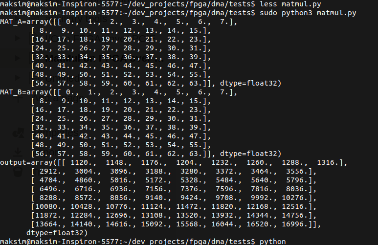
One thing that made figuring this out challenging is that while there’s an abundance of guides that employ the Zynq platform (including the adjacent ARM core functioning as the processor system), there are almost none that discuss accomplishing the goal using other boards/chips/configurations.

TL;DR

If you want to deploy some logic to a FPGA and talk to that logic over PCIE, it’s harder than it has any right to be, but it can be done by gluing together Xilinx’s XDMA core and the logic using AXI. We’ll use memory mapped I/O (MMIO) to actually transfer data from the host to the FPGA.

then you need to generate certs in /lib/modules/$(uname -r)/build/certs (taken from https://superuser.com/a/1322832)

Motivation

Green’s functions are a way to solve certain PDEs. Consider a PDE

A slew of definitions about graphs

A graph \(G\) is a pair \(\left(V,E\right)\) of things: a set \(V\) of vertices and a set \(E\) of edges. Vertices are an abstraction: they can represent anything from cities, people, jobs, classes, etc. to other vertices.

Expectation maximization (EM) is a way to iteratively approximate the maximum likelihood estimators (MLEs) for a parametric family when solving the MLE equations analytically is intractable. Recall that finding the MLEs for a parametric family

is tantamount to maximizing the likelihood function

as a function of \(\boldsymbol{\theta}\).

Quadratic Forms

The gradient of quadratic form

Suppose \(x_{1},x_{2},\dots,x_{n}\) are all quantities drawn, without replacement, a “random” sample, from some population, the same population, which itself has an \(\mathcal{N}\left(\mu,\sigma^{2}\right)\) distribution. If the population size is large enough it’s safe to make the approximation that each draw does not affect the population distribution (despite non-replacement) and so effectively each of the \(x_{i}\) is a draw from an \(\mathcal{N}\left(\mu,\sigma^{2}\right)\) distribution, i.e. each \(x_{i}\) is actually the random variable \(X_{i}\sim\mathcal{N}\left(\mu,\sigma^{2}\right)\). What can we say about the distribution of the random variable \(\bar{X}\equiv\frac{1}{n}\sum_{i=1}^{n}X_{i}\), i.e. the distribution of the “sample mean”? Furthermore what can we say about the distribution of the sample variance \(S^{2}\equiv\frac{1}{n-1}\sum_{i=1}^{n}\left(X_{i}-\bar{X}\right)^{2}\)?

Introduction

Suppose you want to generate a draw of a random variable, i.e. from a distribution of a random variable \(Y\) but the direct method (integral transform, i.e. \(F_{Y}^{-1}\left(U\right)\sim Y\) for \(U\sim\text{uniform}\left(0,1\right)\), which is from \(F_{Y}\left(Y\right)\sim\text{uniform}\left(0,1\right)\)) doesn’t work because you don’t have a closed form for \(F_{Y}\). What do you do?

Most research in quantum computing today is performed against simulations of quantum computers rather than true quantum computers. Simulating a quantum computer entails implementing all of the unitary operators corresponding to the quantum gates as tensors. For high numbers of qubits, performing tensor multiplications for these simulations becomes quite expensive, since $N$-qubit gates correspond to $2^{N}$-dimensional tensors.

High level abstractions for implementing, training, and testing Deep Learning (DL) models abound. Such frameworks function primarily by abstracting away the implementation details of arbitrary neural architectures, thereby enabling researchers and engineers to focus on design. In principle, such frameworks could be “zero-cost abstractions”; in practice, they incur translation and indirection overheads. We study at which points exactly in the engineering life-cycle of a DL model the highest costs are paid and whether they can be mitigated. We train, test, and evaluate a representative DL model using PyTorch, LibTorch, TorchScript, and cuDNN on representative datasets, comparing accuracy, execution time and memory efficiency.

Flame Spray Pyrolysis (FSP) is a manufacturing technique to mass produce engineered nanoparticles for applications in catalysis, energy materials, composites, and more. FSP instruments are highly dependent on a number of adjustable parameters, including fuel injection rate, fuel-oxygen mixtures, and temperature, which can greatly affect the quality, quantity, and properties of the yielded nanoparticles. Optimizing FSP synthesis requires monitoring, analyzing, characterizing, and modifying experimental conditions. Here, we propose a hybrid CPU-GPU Difference of Gaussians (DoG) method for characterizing the volume distribution of unburnt solution, so as to enable near-real-time optimization and steering of FSP experiments. Comparisons against standard implementations show our method to be an order of magnitude more efficient. This surrogate signal can be deployed as a component of an online end-to-end pipeline that maximizes the synthesis yield.

This is a summary of Non-linear protocols for optimal distributed consensus in networks of dynamic agents.

Definitions

• $\Gamma = \{1, \dots, n\}$ is a set of agents/players/nodes/vertices and $G = (\Gamma, E)$ is a fixed (in time) undirected, connected¹, network describing the connections between vertices $i \in \Gamma$, where $E \subset \Gamma \times \Gamma$ is the edge set.
• A neighborhood of a vertex $i$ is the set of all vertices $j$ for which there is a single edge connecting $i,j$, that is to say $N_i := \{j \mid (i,j) \in E\}$.

MinHash is a technique for quickly estimating how similar two sets are.

Definitions

The Jacard index (or Jacard similarity) of two sets $A,B$ is the ratio or the intersection to the union

Notice that $0 \leq J(A,B) \leq 1$ where $J(A,B)=0$ when $A \cap B = \emptyset$ and $J(A,B)=1$ when $A = B$. Let $h$ be a cryptographic hash function¹ and

Note that $h_{\min}(S)$ always exists for a finite set $S$.

Definitions

Markov Decision Process

A Markov Decision Process (MDP) models choosing an action \(a_t\) in an action space \(\mathcal{A}\) while in a state \(s_t\) (from a state space \(\mathcal{S}\)) and thence receiving a reward \(r_t\).

Shannon’s noisy-channel coding theorem

Shannon’s noisy-channel coding theorem sets bounds on how much data can be sent across a noisy channel nearly error free. The Shannon capacity of a channel is the maximum error-free data rate.

Introduction

“Imagine that several divisions of the Byzantine army are camped outside an enemy city, each division commanded by its own general. The generals can communicate with one another only by messenger. After observing the enemy, they must decide upon a common plan of action.

Introduction

Shannon’s source coding theorem accomplishes two things:

Full disclosure: I’m a PhD student in the research group that develops funcX.

Full disclosure: I’m a PhD student in the research group that develops Parsl.

Covariant derivatives are a means of differentiating vectors relative to vectors. First we cover formal definitions of tangent vectors and then proceed to define a means to “covariantly differentiate”.

Covariance and contravariance characterize how quantities (typically vectors) measured in some space transform when the space undergoes a change of basis or coordinate system. A covariant quantity has components that transform in the same way as the basis (to be clarified). A contravariant quantity has components that transform opposite of the basis (to be clarified).

This post follows the series of videos starting with this one and covers derivations of the Black-Scholes model for pricing a European option.

This post makes rigorous the material in the previous two posts (Change of Measure and Girsanov Theorem ).

This post follows this video and this video and covers the intuition for change of measure for a stochastic process and stochastic differential equations.

This post follows this video and covers change of measure for a single Normal random variable.

This post follows this video and explicates Arnold’s topological proof of Abel-Ruffini.

Signal processing is the science of decomposing and transforming signals (for various purposes e.g. study, compression, augmentation, etc).

A game can be thought of as a tree of possible future game states. The current state of the game is the root of the tree (drawn at the top). In general this node has several children, representing all of the possible moves that we could make. Each of those nodes has children representing the game state after each of the opponent’s moves. These nodes have children corresponding to the possible second moves of the current player, and so on. The leaves of the tree are final states of the game: states where no further move can be made because one player has won, or perhaps the game is a tie.

We want to sample from some distribution $P(X)$ in order to be able to calculate empirical expectations of functions $f(X)$ like

A measure $\mu$ on Borel subsets of the real line is absolutely continuous with respect to Lebesgue measure $\lambda$ (in other words, dominated by $\lambda$ ) if for every measurable set $A$, $\lambda(A) = 0$ implies $\mu(A)=0$. This is written as $ \mu \ll \lambda$.

The EM algorithm proceeds by alternatingly taking the expectation of a function $Q$ related to the log-likelihood and maximizing that same function in order to get converging estimates $\theta^{t}$ for some parameter $\theta$. The inspiration is computing the maximum likelihood estimate for some parameter $\theta$ based on some observed data $\left(x_1, x_2, …, x_i, …, x_N\right)$ and some latent variables $\left(z_1, z_2, …, z_i, …, z_N\right)$.

This is a minimal tutorial on Monads i.e. the mechanics rather than the philosophy. I’m not going to convince you that they’re important or beautiful or magical or powerful. On the other hand I will try to convince you that they are simple, that they’re not complicated, abstruse, or impenetrable. All you have to do is unwrap all of the indirection.

Alternatively choose to include and not include element from array and branch (making sure to undo the last move after both branches).

Bit manipulation is useful for things like creating bit sets (which are themselves useful for representing membership efficiently).

Slicker binary search: make jumps and then slow the speed of the jumps when you get closer to the target.

Two sorts that beat $ O \left(n\log n\right) $ complexity.

Functional implementation of Kidane’s for max subarray sum.

Various formulae

Sums of powers