• Sampling
  • Rejection sampling
  • Application to Bayesian inference
  • Adaptive rejection sampling
• Markov Chains
  • Basic Definition
  • Example
  • Some definitions
  • Theorems
    • Equilibrium distributions
    • Reversible Markov Chain
• Interlude
• Metropolis-Hasting
• Gibbs sampling

We want to sample from some distribution $P(X)$ in order to be able to calculate empirical expectations of functions $f(X)$ like

Sampling

Rejection sampling

Imagine plotting the density function $f\left(x\right)$ of a random variable $X$ onto a large rectangular board and throwing darts at it. Assume that the darts are uniformly distributed around the board. Now remove all of the darts that are outside the area under the curve. The remaining darts will be distributed uniformly within the area under the curve, and the $x$-positions of these darts will be distributed according to the random variable’s density. This is because there is the most room for the darts to land where the curve is highest and thus the probability density is greatest.

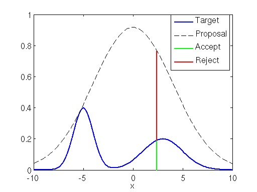
You can be more efficient by using an envelope density rather than just a rectangle. Use a density you can sample from called a “proposal density” $g\left( v \right)$ for a random variable $V$. In fact you can even scale the density of $V$ by $M$: $Mg\left(v\right)$. Then to sample from $X$ you proceed by sampling $v$ from the proposal density (this gives you the position on the $x$-axis) and sampling $U$ uniformly $u \in \left[0, Mg\left(v\right)\right]$. Finally accept the sample if $u < f\left(v\right)$ and reject otherwise. In toto this produces pairs $\left(v, u\right)$ uniformly distributed over the subgraph of $f\left(x\right)$ with $P\left(v\leq x| \mbox{accept}\right) = P_{X}\left(x\right)$:

Note that the density of $U$ is $1/Mg(V)$ and that $U,V$ are independent and hence $p_{U, V} = g(v)/Mg(v) = 1/M$. Hence

Note that because $U$ is uniform this procedure is equivalent to drawing $v$ from the proposal density and then accepting it with probability $f(v)/Mg(v)$ and rejecting with probability $1- f(v)/Mg(v)$ (i.e. flipping a biased coin). This ratio-test-accept-reject is an important sampling paradigm.

Note also that the probability of accepting is

and hence expected acceptance time is related to the geometric distribution i.e. $M$ iterations hence you want to choose $M$ as small as possible (while still satisfying $Mg(v) \geq f(v)$ for all $v$).

If normalizing constants $Z_f, Z_g$ for both distributions $f,g$ are unknown (as in Bayesian inference) rejection sampling still works: just define $M’ = Z_f/MZ_g$ and then $f/g \leq M \iff f’/g’ \leq M’$. Practically this means you can ignore normalizing constants from the start.

Application to Bayesian inference

Suppose we want to draw from the posterior $p\left(\theta | x\right) = p\left(x| \theta \right) p\left(\theta\right)/p\left(x\right)$. We can use rejection sampling with $f(\theta) = p\left(x| \theta \right) p\left(\theta\right)$ as the target distribution and $g(\theta)=p(\theta)$ as the proposal distribution with $M= p(x| \hat{\theta})$ where $\hat{\theta}$ is the MLE. Then we draw from the prior and accept points with probability

Adaptive rejection sampling

There’s an automatic way to come up with a tight envelope density $g(x)$ to any log-concave ¹ density $f(x)$: upper-bound the log-density with a piecewise linear function where initial points of tangency are chosen on a regular grid and the slopes are the gradients of $\log\left[f(x)\right]$ at those grid points. Then $g(x)$ is the piecewise exponential

where $x_i$ are the gridpoints, $M_i$ are determined as usual, and $\lambda_i$ fit the line in log-density space. Sampling from exponential distributions is easy. Further there is refinement to the envelope: if a sample $x$ is rejected then, since we’ve evaluated $f(x)$, we can add another gridpoint and thereby tighten the envelope.

Markov Chains

Basic Definition

A Markov chain is a stochastic model describing a sequence of possible events in which the probability of each event depends only on the state attained in the previous event, i.e. in the discrete case

Markov chains are often described by a sequence of directed graphs, where the edges of the graph are labeled by the probabilities of going from one state at time $n$ to the other states at time $n + 1$, $ P(X_{n+1}=x\mid X_{n}=x_{n})$. The same information is represented by the transition matrix from time $n$ to time $n + 1$. Time-homogeneous Markov chains (or stationary Markov chains) are processes where

i.e. for all times $n$ the probability of the transition is independent of $n$.

Example

Here is an example modeling a hypothetical stock market

Labelling the state space {1 = bull, 2 = bear, 3 = stagnant} the transition matrix for this example is

Using the transition matrix it is possible to calculate, for example, the long-term fraction of weeks during which the market is stagnant, or the average number of weeks it will take to go from a stagnant to a bull market. Using the transition probabilities, the steady-state probabilities indicate that 62.5% of weeks will be in a bull market, 31.25% of weeks will be in a bear market and 6.25% of weeks will be stagnant, since:

Some definitions

• A Markov chain is said to be irreducible if it is possible to get to any state from any state i.e. the underlying directed graph is strongly connected.

• A state i is said to be transient if, given that we start in state i, there is a non-zero probability that we will never return to i. State i is recurrent (or persistent) if it is not transient. Recurrent states are guaranteed (with probability 1) to have a finite hitting time. This is equivalent to the state being in a strongly connected (irreducible) component with no outgoing edges. Even if the hitting time is finite with probability 1, it need not have a finite expectation. The mean recurrence time at state i is the expected return time $M_i$:

  \[{\displaystyle M_{i}=E[T_{i}]=\sum _{n=1}^{\infty }n\cdot f_{ii}^{(n)}.}\]

  State i is positive recurrent (or non-null persistent) if $M_i$ is finite; otherwise, state i is null recurrent (or null persistent).

• A state i has period k if any return to state i must occur in multiples of k time steps. Formally, the period of a state is defined as

  \[k=\gcd\{n>0:P(X_{n}=i\mid X_{0}=i)>0\}\]

  provided that this set is not empty. Otherwise the period is not defined. If k = 1, then the state is said to be aperiodic. Otherwise (k > 1), the state is said to be periodic with period k. A Markov chain is aperiodic if every state is aperiodic i.e. the $\gcd$ of $\gcd$s of all lengths of all directed cycles in the graph is 1. A strongly connected (irreducible) Markov chain only needs one aperiodic state to imply all states are aperiodic (obvious since $\gcd$ of any set that contains 1 is 1).

• A state i is said to be ergodic (random) if it is aperiodic and positive recurrent. In other words, a state i is ergodic if it is recurrent, has a period of 1, and has finite mean recurrence time. If all states in an irreducible Markov chain are ergodic, then the chain is said to be ergodic.

• If the Markov chain is a time-homogeneous Markov chain, so that the process is described by a single, time-independent matrix , then the vector $\pi$ is called a stationary distribution (or invariant measure) if ${\displaystyle \forall j\in S}$ it satisfies

  \[\begin{eqnarray} 0\leq \pi _{j}\leq 1 \nonumber \\ \sum _{j\in S}\pi _{j}=1 \nonumber \\ \pi _{j}=\sum _{i\in S}\pi _{i}p_{ij} \nonumber\\ \end{eqnarray}\]

• A Markov chain is said to be reversible if there is a probability distribution $\pi$ over its states such that \(\pi _{i}P(X_{n+1}=j\mid X_{n}=i)=\pi _{j}P(X_{n+1}=i\mid X_{n}=j)\)

  for all times n and all states i and j. This condition is known as the detailed balance condition (some books call it the local balance equation).

Theorems

Equilibrium distributions

An irreducible chain has a positive stationary distribution (a stationary distribution such that ${\displaystyle \forall i,\pi _{i}>0}$ ) if and only if all of its states are positive recurrent. In that case, $\pi$ is unique and is related to the expected return time:

where $C$ is the normalizing constant. Further, if the positive recurrent chain is both irreducible and aperiodic, it is said to have a limiting distribution; for any i and j

where $p_{ij}^{(n)}=P(X_{n+1}=j\mid X_{n}=i)$. There is no assumption on the starting distribution; the chain converges to the limiting distribution regardless of where it begins. Such $\pi$ is called the equilibrium distribution of the chain.

Reversible Markov Chain

Considering a fixed arbitrary time n and using the shorthand

Then the detailed balance condition can be written more compactly as

Note that

As $n$ was arbitrary, this reasoning holds for any $n$, and therefore for reversible Markov chains $\pi$ is always a steady-state distribution for every $n$.

Reversible Markov chains are common in MCMC because satisfying the detailed balance condition for a desired distribution $\pi$ necessarily implies that the Markov chain has been constructed so that $\pi$ is a stationary distribution.

Interlude

For our purposes, the key idea of MCMC is to think of $X$’s as points in a state space and to find ways to “walk around” the space — going from $X_0$ to $X_1$ to $X_2$ and so forth — so that the likelihood of visiting any point $X$ is proportional to $P(X)$. A walk of this kind can be characterized abstractly as follows:

$X_0 \gets$ random()
for $t = 1$ to $T$:
    $X_{t+1} \gets g\left( X_t \right)$

Here $g$ is a function that makes a probabilistic choice about what state to go to next according to an explicit or implicit transition probability \(P_{\mbox{trans}}\left(X_{t+1}|X_0, X_1, \dots , X_t\right)\)

One way to implement this plan (where the state space walk spends most of its time in areas of high $P(X)$) is to construct a Markov chain since the chain will naturally spend most of its time in such areas (if the chain has a stationary distribution and it’s aperiodic).

Therefore the heart of Markov Chain Monte Carlo methods is designing a chain so that the probability of visiting a state $X$ will turn out to be $P(X)$, as desired. This can be accomplished by guaranteeing that the chain, as defined by the transition probabilities $P_{\mbox{trans}}$, meets certain conditions.

Metropolis-Hasting and Gibbs sampling are two algorithms that meet those conditions.

Metropolis-Hasting

Start with a connected undirected graph $G$ on a set of states. If the states are the lattice points $\left(x_1, x_2, \dots, x_d \right) \in \mathbb{R}^d$ with $x_i \in {0, 1, \dots, n}$, then $G$ could be the lattice graph with $2d$ coordinate edges at each interior vertex. In general, let $r$ be the maximum degree of any vertex of $G$. The transitions of the Markov chain are defined as follows: at state i select neighbor j with probability $\frac{1}{r}$. Since the degree of i may be less than $r$, with some probability no edge is selected and the walk remains at vertex i. If a neighbor j is selected and $p_j \geq p_i$ then go to j. Otherwise ($p_j < p _i$) go to j with probability $p_j / p_i$ and stay at i with probability $1- \frac{p_j}{p_i}$. Intuitively, this favors “heavier” states with higher $p$ values. In summary \(p_{ij} = \frac{1}{r} \min \left(1, \frac{p_j}{p_i} \right)\) and \(p_{ii} = 1- \sum_\limits{j\neq i} p_{ij}\) Thus \(p_i p_{ij} = \frac{p_i}{r} \min \left(1, \frac{p_j}{p_i} \right) = \frac{1}{r} \min \left(p_i, p_j \right) = \frac{p_j}{r} \min \left(1, \frac{p_i}{p_j} \right) = p_j p_{ji}\) and therefore the chain satisfies the detailed balance condition and hence the stationary distribution of the Markov chain is $p_i$ as desired.

Gibbs sampling

Let $p(\textbf{x})$ be the target distribution, where $\textbf{x} = \left(x_1, x_2, \dots, x_d \right)$. Gibbs sampling consists of a random walk on an undirected graph whose vertices correspond to the values $\textbf{x} = \left(x_1, x_2, \dots, x_d \right)$ and in which there’s an edge from $\textbf{x}$ to $\textbf{y}$ if $\textbf{x}$ and $\textbf{y}$ differ in only one coordinate. Thus, the underlying graph is like a $d$-dimensional lattice except that the vertices in the same coordinate line form a clique.

To generate samples of the target distribution, the Gibbs algorithm repeats the following steps: one of the coordinates $x_i$ is chosen to be updated and its new value is chosen based on the marginal probability of $x_i$ with the other coordinates fixed. There are two commonly used schemes to determine which $x_i$ to update: either choose $x_i$ randomly or by scanning sequentially from $x_1$ to $x_d$.

Now suppose that $\textbf{x}$ and $\textbf{y}$ differ in only one coordinate. Without loss of generality that coordinate (that which they differ in) be $x_1$. Then, in the scheme where a coordinate is chosen randomly the probability $p_{\textbf{x}\textbf{y}}$ of going from $\textbf{x}$ to $\textbf{y}$ is

The normalizing constant is $1/d$ since $\sum\limits_{y_1} p\left(y_1 |x_2, x_3, \dots, x_d \right) = 1$ and summing over $d$ coordinates

Similarly

where we have used that for $j\neq 1$, $x_j =y_j$. Then we can see that this chain has a stationary distribution proportional to $p\left( \textbf{x} \right)$

again using that for $j\neq 1$, $x_j =y_j$. Similarly

from which it follows that $p\left(\textbf{x}\right) p_{\textbf{x}\textbf{y}}= p\left(\textbf{y}\right) p_{\textbf{y}\textbf{x}}$ and hence the chain satisfies the detailed balance condition and hence the stationary distribution of the Markov chain is $p_i$ as desired.

1. For strictly positive $f$ : $ \log\left[f(\theta x+(1-\theta )y)\right]\geq \theta \log\left[f(x)\right]+ \left(1-\theta\right) \log\left[f(y)\right]$