• Motivation
• Green’s function for the Diffusion equation
• Smoothing
• Footnotes

Motivation

Green’s functions are a way to solve certain PDEs. Consider a PDE

\[\begin{align} \frac{\partial u}{\partial t}-\frac{D}{2}\frac{\partial^{2}u}{\partial x^{2}} & =\left(\frac{\partial}{\partial t}-\frac{D}{2}\frac{\partial^{2}}{\partial x^{2}}\right)\label{eq:diffeqn}\\ & =Lu\label{eq:pdesystem} \\ u\left(x,0\right) & =f\left(x\right)\nonumber \end{align}\]

as a linear system¹ \(L\) with input \(f\left(x\right)\) and response \(u\). This is appropriate because \(u\left(x,t\right)\) is completely characterized² by \(L\) and \(f\left(x\right)\). The Green’s function \(G\left(x,t\right)\) of the system is the solution that satisfies

\[\lim_{t\downarrow0}G\left(x,t\right)=\delta\left(x\right)\label{eq:initcondimpul}\]

Note that this is the impulse response of the system because it is the response/solution of the system whose input/initial conditions \(u\left(x,0\right)=G\left(x,0\right)\) are in a sense³ the unit impulse \(\delta\left(x\right)\). Why is the Green’s function useful? For arbitrary⁴ input \(f\left(x\right)\)

\[\begin{align} L\left(\int_{-\infty}^{\infty}G\left(s-x,t\right)f\left(s\right)ds\right) & =\int_{-\infty}^{\infty}\left[LG\left(s-x,t\right)\right]f\left(s\right)ds\\ & =\int_{-\infty}^{\infty}\left[\frac{\partial G}{\partial t}-\frac{D}{2}\frac{\partial^{2}G}{\partial x^{2}}\right]f\left(s\right)ds\\ & =0\end{align}\]

and

\[\begin{align} \lim_{t\downarrow0}\left(\int_{-\infty}^{\infty}G\left(s-x,t\right)f\left(s\right)ds\right) & =\int_{-\infty}^{\infty}\left[\lim_{t\downarrow0}G\left(s-x,t\right)\right]f\left(s\right)ds\nonumber \\ & =\int_{-\infty}^{\infty}\delta\left(s-x\right)f\left(s\right)ds\label{eq:siftprop}\\ & =f\left(x\right)\nonumber \end{align}\]

So

\[\begin{align} u\left(x,t\right) & =\int_{-\infty}^{\infty}G\left(s-x,t\right)f\left(s\right)ds\\ & =G\left(x,t\right)\star f\left(x\right)\end{align}\]

is a general solution of the system defined by eqns. \(\eqref{eq:pdesystem}\).

Green’s function for the Diffusion equation

The PDE in eqn. \(\eqref{eq:diffeqn}\) is called the Diffusion equation and the system I’ll call a Diffusion system⁵: it diffuses the initial concentration of mass \(f\left(x\right)\) as time evolves. We seek a general solution to the system and therefore we seek the Green’s function \(G\left(x,t\right)\) for the system. For reasons that will become clearer in the 3rd section

\[\begin{align} G\left(x,t\right) & =\frac{1}{t^{\alpha}}\phi\left(\frac{x}{t^{\alpha}}\right)\label{eq:greenprototype}\end{align}\]

for any smooth⁶ and integrable function \(\phi\left(y\right)\) is a good guess for the form of a Green’s function. Indeed we will construct \(G\) by finding a suitable \(\phi\). Substituting this \(G\) into the diffusion equation

\[\begin{align} \frac{\partial G}{\partial t}-\frac{D}{2}\frac{\partial^{2}G}{\partial x^{2}} & =\left(-\frac{\alpha}{t^{\alpha+1}}\phi-\frac{\alpha x}{t^{2\alpha+1}}\phi'\right)-\frac{D}{2}\left(\frac{1}{t^{3\alpha}}\phi''\right)\label{eq:greeneqn}\end{align}\]

To simplify the notation a little define \(\eta\left(x\right)=\phi\left(\frac{x}{t^{\alpha}}\right)\). Then

\[\begin{align} \eta'\left(x\right) & =\frac{1}{t^{\alpha}}\phi'\left(x\right)\\ \eta''\left(x\right) & =\frac{1}{t^{2\alpha}}\phi''\left(x\right)\end{align}\]

and eqn. \(\eqref{eq:greeneqn}\) becomes

\[\left(-\frac{\alpha}{t^{\alpha+1}}\eta\left(x\right)-\frac{\alpha x}{t^{\alpha+1}}\eta'\left(x\right)\right)-\frac{D}{2}\left(\frac{1}{t^{\alpha}}\eta''\left(x\right)\right)=0\]

or (by multiplying both sides by \(-t^{\alpha}/\left(D/2\right)\) and moving \(\eta''\left(x\right)\) over)

\[\frac{\alpha}{\left(D/2\right)t}\eta\left(x\right)+\frac{\alpha x}{\left(D/2\right)t}\eta'\left(x\right)=-\eta''\left(x\right)\label{eq:odegreen}\]

This is now a linear second order ordinary differential equation that’s easy to solve. The first trick is recognizing the left side is an exact differential, i.e.

\[\frac{\alpha}{\left(D/2\right)t}\eta\left(x\right)+\frac{\alpha x}{\left(D/2\right)t}\eta'\left(x\right)=\frac{\alpha}{\left(D/2\right)t}\frac{d}{dx}\left(x\eta\left(x\right)\right)\]

and hence eqn. \(\eqref{eq:odegreen}\) can be integrated once easily

\[\begin{align} \frac{\alpha}{\left(D/2\right)t}\int\frac{d}{dx}\left(x\eta\left(x\right)\right) & =-\int\eta''\left(x\right)dx\\ \frac{\alpha}{\left(D/2\right)t}x\eta\left(x\right) & =-n'\left(x\right)+c_{1}\end{align}\]

This again is a linear first order ordinary differential equation more commonly written

\[n'\left(x\right)+\frac{\alpha x}{\left(D/2\right)t}\eta\left(x\right)=c_{1}\]

which is solved by a similar sort of trick. The left side is almost an exact differential⁷ except the \(x\) spoils it. We can hack it to indeed be an exact differential by multiplying both sides by some function \(h\left(x\right)\)

\[\left[h\left(x\right)\right]n'\left(x\right)+\left[h\left(x\right)\frac{\alpha x}{\left(D/2\right)t}\right]\eta\left(x\right)=h\left(x\right)c_{1}\label{eq:integfac}\]

such that the second term becomes the first derivative of \(h\), i.e.

\[h\left(x\right)n'\left(x\right)+h'\left(x\right)\eta\left(x\right)=\frac{d}{dx}\left(h\left(x\right)\eta\left(x\right)\right)\]

Which function has the property that it’s first derivative is equal to itself times \(\alpha x/\left(D/2\right)t\)? Well that’s just another⁸ differential equation in disguise!

\[\frac{dh}{dx}=h\cdot\frac{\alpha x}{\left(D/2\right)t}\Rightarrow\frac{dh}{h}=dx\frac{\alpha x}{\left(D/2\right)t}\Rightarrow\log\left(h\right)=\frac{\alpha}{Dt}x^{2}\]

or \(h\left(x\right)=e^{\alpha x^{2}/Dt}\). So substituting \(h\) into eqn. \(\eqref{eq:integfac}\)

\[\frac{d}{dx}\left(e^{\alpha x^{2}/Dt}\eta\left(x\right)\right)=e^{\alpha x^{2}/Dt}c_{1}\]

and finally

\[\begin{align} e^{\frac{\alpha x^{2}}{Dt}}\eta\left(x\right) & =c_{1}\int e^{\alpha x^{2}/Dt}dx+c_{2}\\ & \text{or}\\ \phi\left(\frac{x}{t^{\alpha}}\right)=\eta\left(x\right) & =c_{1}e^{-\frac{\alpha x^{2}}{Dt}}\int e^{\alpha x^{2}/Dt}dx+c_{2}e^{-\frac{\alpha x^{2}}{Dt}}\end{align}\]

Now to reconcile that \(\phi\left(\frac{x}{t^{\alpha}}\right)\) should be a function of only \(\frac{x}{t^{\alpha}}\) we need to pick the appropriate \(\alpha\). Inspect that for \(\alpha=1/2\)

\[\phi\left(\frac{x}{\sqrt{t}}\right)=c_{1}e^{-\frac{1}{2D}\left(\frac{x}{\sqrt{t}}\right)^{2}}\int e^{\frac{1}{2D}\left(\frac{x}{\sqrt{t}}\right)^{2}}dx+c_{2}e^{-\frac{1}{2D}\left(\frac{x}{\sqrt{t}}\right)^{2}}\]

So \(\phi\left(\frac{x}{\sqrt{t}}\right)\) is the Green’s function of the diffusion equation. Well almost. The regularity conditions mentioned in footnote [fn:Given-some-regularity] require that \(\phi\rightarrow0\) as \(x\rightarrow\infty\) and for the calculation in eqns. \(\eqref{eq:siftprop}\) to work \(G\) should be normalized to integrate to 1. To satisfy the first requirement it’s clear that \(c_{1}\) should be 0. To meet the second requirement we set \(c_{2}\):

\[\begin{align} 1 & =\int_{-\infty}^{\infty}G\left(x,t\right)dx\\ & =c_{2}\int_{-\infty}^{\infty}\frac{1}{\sqrt{t}}e^{-\frac{1}{2D}\left(\frac{x}{\sqrt{t}}\right)^{2}}dx\\ & =c_{2}\int_{-\infty}^{\infty}\frac{1}{\sqrt{t}}e^{-\frac{1}{2}\left(\frac{x}{\sqrt{Dt}}\right)^{2}}dx\\ & \text{let }u=x/\sqrt{Dt}\\ & =c_{2}\sqrt{D}\int_{-\infty}^{\infty}e^{-\frac{1}{2}u^{2}}du\\ & =c_{2}\sqrt{2D\pi}\end{align}\]

Therefore the normalization factor \(c_{2}=1/\sqrt{D\pi}\) and the complete Green’s function is

\[G\left(x,t\right)=\frac{1}{\sqrt{2\pi Dt}}e^{-\frac{1}{2}\frac{x^{2}}{Dt}}\label{eq:gaussian}\]

Indeed a very recognizable function! And hence the general solution to the diffusion equation is

\[\begin{align} u\left(x,t\right) & =\int_{-\infty}^{\infty}G\left(s-x,t\right)f\left(s\right)ds\\ & =\frac{1}{\sqrt{2\pi t}}\int_{-\infty}^{\infty}\frac{1}{\sqrt{t}}e^{-\frac{1}{2}\frac{\left(s-x\right)^{2}}{Dt}}f\left(s\right)ds\end{align}\]

Smoothing

A Green’s function is a smoother⁹ and \(u\left(x,t\right)\) is the smoothed version of \(f\left(x\right)\). Figure 1 shows initial conditions \(f\left(x\right)\) for

\[f\left(x\right)=\begin{cases} 0 & x<-1\\ x+1 & -1\leq x<0\\ 1 & 0\leq x<1\\ 2 & 1\leq x<2\\ 0 & 2\leq x \end{cases}\]

and \(G\left(x,t\right)\) convolved with \(f\left(x\right)\) for \(t=.01,.1,1\), i.e. the solution \(u\left(x,t\right)\) to the diffusion equation at those times. As you can see as \(t\) increases the initial distribution of mass \(f\left(x\right)\) is diffused out and the points where \(f\left(x\right)\) is nondifferentiable¹⁰ vanish, i.e. \(u\left(x,t\right)\) is differentiable at those points.

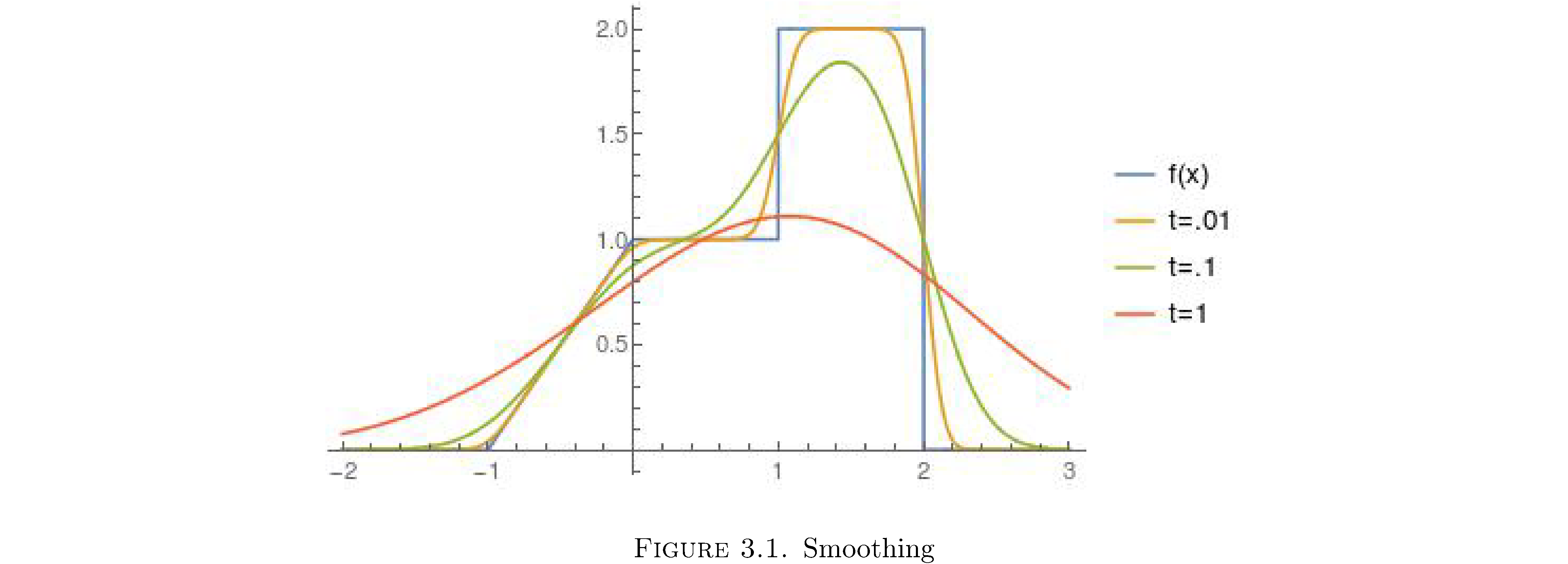
Actually \(u\left(x,t\right)\) is \(C^{\infty}\) for any \(t>0\), so \(f\left(x\right)\) is instaneously smoothed out. How smooth? Perfectly smooth:

\[\begin{align} \frac{\partial^{n}}{\partial x^{n}}u\left(x,t\right) & =\int_{-\infty}^{\infty}\left(\frac{\partial^{n}}{\partial x^{n}}G\left(s-x,t\right)\right)f\left(s\right)ds\\ & =\int_{-\infty}^{\infty}\left(-1\right)^{n}G^{\left(n\right)}\left(s-x,t\right)f\left(s\right)ds\end{align}\]

where \(G^{\left(n\right)}\) denotes the \(n\)th partial deriviative of \(G\) with respect to its first argument. And since \(G\left(x,t\right)\) is \(C^{\infty}\)¹¹ this integral converges for all \(n\). Even more shockingly \(u\left(x,t\right)\) is non-zero everywhere on \(\mathbb{R}\) for any \(t>0\), so \(f\left(x\right)\) is diffused everywhere instaneously.

Why is that eqn. \(\eqref{eq:greenprototype}\)

\[G\left(x,t\right)=\frac{1}{t^{\alpha}}\phi\left(\frac{x}{t^{\alpha}}\right)\]

is a good guess for the form a Green’s function? First of all first of all since \(\phi\) is integrable we can normalize it such that

\[\int_{-\infty}^{\infty}\phi\left(y\right)dy=1\]

and then by a change of variables

\[\int_{-\infty}^{\infty}\frac{1}{t^{\alpha}}\phi\left(\frac{x}{t^{\alpha}}\right)dx=1\]

which as already mentioned is necessary for the calcuation in eqns. \(\eqref{eq:siftprop}\) to work.

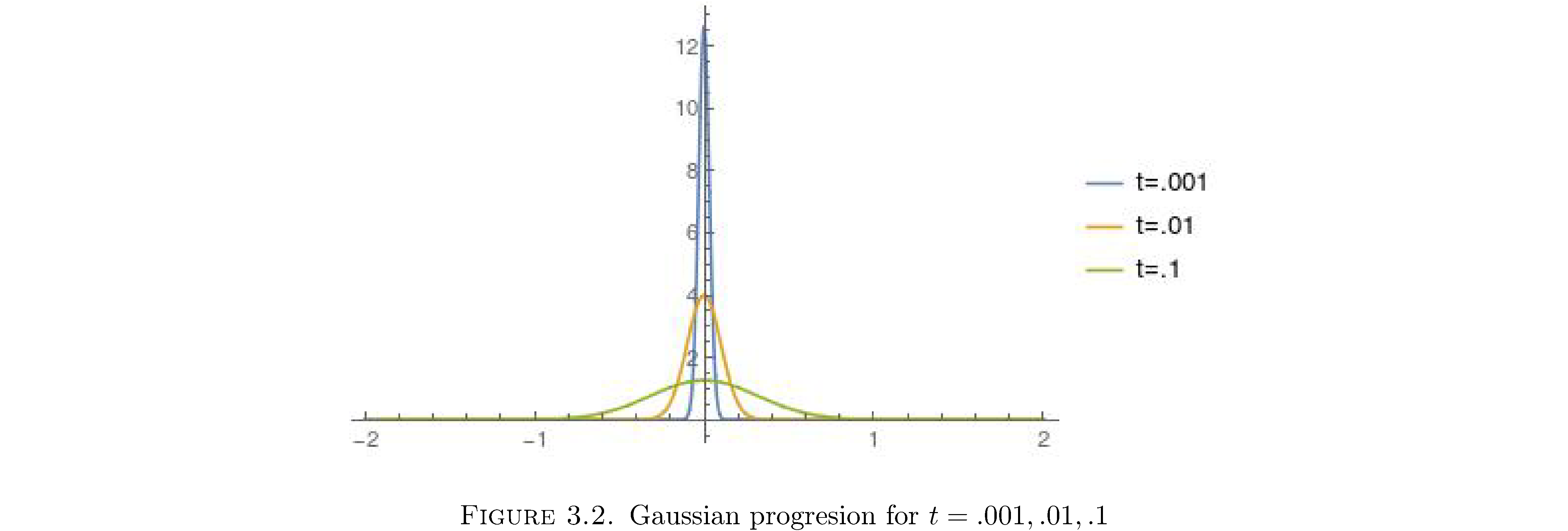
But more intuitively eqn. \(\eqref{eq:greenprototype}\) is the right form for a Green’s function because it has the behavior of a smoother as \(t\rightarrow0\) and as \(t\rightarrow\infty\). As \(t\rightarrow0\) the the factor of \(1/t^{\alpha}\) increases the value of \(G\left(x,t\right)\) around \(x=0\) and shrinks the base because the \(1/t^{\alpha}\) in the argument of \(\phi\) functions as a scale parameter¹². So initially (at \(t\approx0\)) a \(G\) of this form will preserve the initial distribution of mass \(f\left(x\right)\). As \(t\rightarrow\infty\) the inverse effect on \(G\left(x,t\right)\) is observed: the factor \(1/t^{\alpha}\) will flatten \(G\left(x,t\right)\) and therefore spread/smear/smooth out \(f\left(x\right)\). It’s also critical that \(G\left(x,t\right)\) integrates to 1 because otherwise it would add mass to the initial distribution¹³and that’s not. My point here is that if you wanted to construct a smoothing function de-noveau you would want these properties and the \(1/t^{\alpha}\) trick would be an easy way to effect them. Figure 2 shows what the Green’s function for the diffusion equation, eqn. \(\eqref{eq:gaussian}\), looks like as \(t\) increases.

Footnotes