• Expectation Maximization Beta
• Expectation Maximization for Real
• Applications
  • Gaussian Mixture Models
• References
• Footnotes

Expectation maximization (EM) is a way to iteratively approximate the maximum likelihood estimators (MLEs) for a parametric family when solving the MLE equations analytically is intractable. Recall that finding the MLEs for a parametric family

\[\mathbf{Y}\sim f_{\mathbf{Y}}\left(\cdot;\boldsymbol{\theta}\right)\,\boldsymbol{\theta}\in\Theta\]

is tantamount to maximizing the likelihood function

\[L\left(\boldsymbol{\theta};\mathbf{y}\right)=f_{\mathbf{Y}}\left(\mathbf{y};\boldsymbol{\theta}\right)\]

as a function of \(\boldsymbol{\theta}\). The maximum likelihood estimators are estimators of/for \(\boldsymbol{\theta}\), usually denoted \(\hat{\boldsymbol{\theta}}\). The actual maximization is effected by finding critical points of \(L\) with respect to \(\boldsymbol{\theta}\) and testing concavity, i.e. solving

\[\nabla L\left(\boldsymbol{\theta};\mathbf{y}\right)=0\]

and checking the negative definiteness of Hessian of \(L\). In general \(\partial_{\theta_{i}}L\left(\boldsymbol{\theta};\mathbf{y}\right)\) might be highly non-linear in \(\theta_{i}\) and hence finding each might be very difficult. What to do?

Expectation Maximization Beta

Suppose¹ there exists another random, unobserved, vector \(\mathbf{X}\) such that were \(\mathbf{X}\) in fact observed, maximizing the joint likelihood for \(\mathbf{X}\) and \(\mathbf{Y}\)

\[L\left(\boldsymbol{\theta};\mathbf{x},\mathbf{y}\right)=f_{\mathbf{X},\mathbf{Y}}\left(\mathbf{x},\mathbf{y};\boldsymbol{\theta}\right)\]

is easier than the original problem. \(\mathbf{X}\) is called a latent or hidden variable. Now a priori there’s absolutely no reason to assume that having more information in hand and complicating the model should make things easier. On the contrary, for example, a good physical model makes simplifying assumptions and thereby becomes tractable. But indeed for some very useful models such as Hidden Markov Models and Gaussian Mixture Models this ansatz does simplify computing the MLEs.

All is going swimmingly except \(\mathbf{X}\) is unobserved - the only observed data are \(\mathbf{Y}\). What to do? Estimate \(\mathbf{X}\) of course. How? Using the best estimator \(E\left[\mathbf{X}|\mathbf{y};\boldsymbol{\theta}\right]\) of \(\mathbf{X}\), based on observed \(\mathbf{y}\), that minimizes the risk for the quadratic loss function², i.e. minimizes the mean square error. Note two things. Firstly, it’s important that you can actually compute this in closed form, otherwise you’ve traded one intractable problem for another. Secondly, since \(E\left[\mathbf{X}|\mathbf{y};\boldsymbol{\theta}\right]\) is implicitly a function of \(\boldsymbol{\theta}\), which is unknown to begin with³ you need some initial guess for it too, otherwise you can’t compute the expectation. Hence the expectation computed is actually \(E\left[\mathbf{X}|\mathbf{y};\boldsymbol{\theta}^{\left(r\right)}\right]\) where \(\boldsymbol{\theta}^{\left(r\right)}\) is the current guess for \(\boldsymbol{\theta}\). Then once you have this estimate for \(\mathbf{X}\) just maximize

\[L\left(\boldsymbol{\theta};E\left[\mathbf{X}|\mathbf{y};\boldsymbol{\theta}^{\left(r\right)}\right],\mathbf{y}\right)=f_{\mathbf{X},\mathbf{Y}}\left(E\left[\mathbf{X}|\mathbf{y};\boldsymbol{\theta}^{\left(r\right)}\right],\mathbf{y};\boldsymbol{\theta}\right)\]

The procedure alternates between estimating x using \(E\left[\mathbf{X}|\mathbf{y};\boldsymbol{\theta}^{\left(r\right)}\right]\) and maximizing \(L\left(\boldsymbol{\theta};E\left[\mathbf{X}|\mathbf{y};\boldsymbol{\theta}^{\left(r\right)}\right],\mathbf{y}\right)\). Compute expectation, then perform maxization, compute expectation, then perform maximization, compute expectation,… hence Expectation Maximization algorithm. Just to be clear

Expectation Algorithm Beta. Given some observed data \(\mathbf{y}\), in order to perform the intractable maximization of \(L\left(\boldsymbol{\theta};\mathbf{y}\right)\), posit the existence of some latent \(\mathbf{x}\) such that \(L\left(\boldsymbol{\theta};\mathbf{x},\mathbf{y}\right)\) is easier. Set \(\boldsymbol{\theta}^{\left(0\right)}\) to be some initial guess for \(\boldsymbol{\theta}\) then

1. E-step: Set \(\mathbf{x}^{\left(r\right)}=E\left[\mathbf{X}|\mathbf{y};\boldsymbol{\theta}^{\left(r\right)}\right]\)

   1. M-step: Set \(\boldsymbol{\theta}^{\left(r+1\right)}=\arg\max_{\boldsymbol{\theta}}L\left(\boldsymbol{\theta};\mathbf{x}^{\left(r\right)},\mathbf{y}\right)\)

   2. Go to step 1 unless \(\left|\boldsymbol{\theta}^{\left(r+1\right)}-\boldsymbol{\theta}^{\left(r\right)}\right|<\varepsilon\) for some \(\varepsilon\) of your choosing.

The equations in step 1 and 2 are called update equations because specify how to update the current estimate for \(\mathbf{x}^{\left(i\right)}\) and \(\boldsymbol{\theta}^{\left(i\right)}\).

Here’s an example: let \(Y_{i}\) be iid such that

\[f_{Y_{i}}\left(y_{i};\theta\right)=\theta g_{1}\left(y_{i}\right)+\left(1-\theta\right)g_{0}\left(y_{i}\right)\]

where \(\theta\in\left(0,1\right)\) and \(g_{0}\) and \(g_{1}\) are Gaussians with known means \(\left(\mu_{0},\mu_{1}\right)\)and variances \(\left(\sigma_{0}^{2},\sigma_{1}^{2}\right)\). We want the MLE for \(\theta\). Note that

\[L\left(\theta;\mathbf{y}\right)=\prod_{i=1}^{n}\left(\theta g_{1}\left(y_{i}\right)+\left(1-\theta\right)g_{0}\left(y_{i}\right)\right)\]

Quite messy⁴. What to do? EM to the rescue! Suppose the \(Y_{i}\) are drawn by a process where a \(\theta\)-biased coin is flipped and either \(g_{0}\) or \(g_{1}\) generates the \(y_{i}\) depending on whether the coin lands heads up or down. The latent variable here then is which Gaussian generated \(y_{i}\). Hence let \(X_{i}\) be Bernoulli random variables where

\[\begin{align} P\left(X_{i}=x_{i}\right) & =\begin{cases} \theta & \text{ if }x_{i}=1\\ 1-\theta & \text{ if }x_{i}=0 \end{cases}\\ & =\theta^{x_{i}}\left(1-\theta\right)^{1-x_{i}}\end{align}\]

and \(f_{Y_{i}|X_{i}}\left(y_{i}|x_{i}=1;\theta\right)=g_{1}\left(y_{i}\right)\) and \(f_{Y_{i}|X_{i}}\left(y_{i}|x_{i}=0;\theta\right)=g_{0}\left(y_{i}\right)\). Then

\[f_{X_{i},Y_{i}}\left(x_{i},y_{i};\theta\right)=f_{Y_{i}|X_{i}}\left(y_{i}|x_{i};\theta\right)P\left(X_{i}=x_{i}\right)\]

and so

\[\begin{align} L\left(\theta;\mathbf{x},\mathbf{y}\right) & =\prod_{i=1}^{n}f_{Y_{i}|X_{i}}\left(y_{i}|x_{i};\theta\right)P\left(X_{i}=x_{i}\right)\\ & =\prod_{i=1}^{n}\left(g_{1}\left(y_{i}\right)\right)^{x_{i}}\left(g_{0}\left(y_{i}\right)\right)^{1-x_{i}}\theta^{x_{i}}\left(1-\theta\right)^{1-x_{i}}\\ & =\theta^{\sum_{i}x_{i}}\left(1-\theta\right)^{n-\sum_{i}x_{i}}\prod_{i=1}^{n}\left(g_{1}\left(y_{i}\right)\right)^{x_{i}}\left(g_{0}\left(y_{i}\right)\right)^{1-x_{i}}\end{align}\]

Note the trick in writing \(f_{Y_{i}|X_{i}}\left(y_{i}|x_{i};\theta\right)=\left(g_{1}\right)^{x_{i}}\left(g_{0}\right)^{1-x_{i}}\)

• it comes up a lot for a class of models called mixture models. For the E-step, to compute \(E\left[\mathbf{X}|\mathbf{y};\theta'\right]\) we use i.i.d-ness and compute \(E\left[X_{i}|y_{i};\theta'\right]\) instead, which will hold for each \(i\). To compute the conditional expectation \(E\left[X_{i}|y_{i};\theta\right]\) we need the conditional distribution \(f_{X_{i}|Y_{i}}\left(x_{i}|y_{i}\right)\). By Bayes’ Theorem

\[\begin{align} f_{X_{i}|Y_{i}}\left(x_{i}|y_{i};\theta\right) & =\frac{f_{X_{i},Y_{i}}\left(x_{i},y_{i};\theta\right)}{f_{Y_{i}}\left(y_{i};\theta\right)}\\ & =\frac{f_{X_{i},Y_{i}}\left(x_{i},y_{i};\theta\right)}{\sum_{x_{i}}f_{X_{i},Y_{i}}\left(x_{i},y_{i};\theta\right)}\\ & =\frac{\left(g_{1}\left(y_{i}\right)\right)^{x_{i}}\left(g_{0}\left(y_{i}\right)\right)^{1-x_{i}}\theta^{x_{i}}\left(1-\theta\right)^{1-x_{i}}}{\sum_{x_{i}}\left(g_{1}\left(y_{i}\right)\right)^{x_{i}}\left(g_{0}\left(y_{i}\right)\right)^{1-x_{i}}\theta^{x_{i}}\left(1-\theta\right)^{1-x_{i}}}\\ & =\frac{\left(g_{1}\left(y_{i}\right)\right)^{x_{i}}\left(g_{0}\left(y_{i}\right)\right)^{1-x_{i}}\theta^{x_{i}}\left(1-\theta\right)^{1-x_{i}}}{g_{1}\left(y_{i}\right)\theta+g_{0}\left(y_{i}\right)\left(1-\theta\right)}\\ & =\left(\frac{g_{1}\left(y_{i}\right)\theta}{g_{1}\left(y_{i}\right)\theta+g_{0}\left(y_{i}\right)\left(1-\theta\right)}\right)^{x_{i}}\left(\frac{g_{0}\left(y_{i}\right)\left(1-\theta\right)}{g_{1}\left(y_{i}\right)\theta+g_{0}\left(y_{i}\right)\left(1-\theta\right)}\right)^{1-x_{i}}\end{align}\]

So \(X_{i}\mid Y_{i}\) is still Bernoulli just renormalized. Hence

\[E\left[X_{i}|y_{i};\theta\right]=\frac{g_{1}\left(y_{i}\right)\theta}{g_{1}\left(y_{i}\right)\theta+g_{0}\left(y_{i}\right)\left(1-\theta\right)}\]

For the M-step, since

\[\begin{align} L\left(\theta;\mathbf{x},\mathbf{y}\right) & = & \left[\theta^{\sum_{i}x_{i}}\left(1-\theta\right)^{n-\sum_{i}x_{i}}\right]\left[\prod_{i=1}^{n}\left(g_{1}\left(y_{i}\right)\right)^{x_{i}}\left(g_{0}\left(y_{i}\right)\right)^{1-x_{i}}\right]\end{align}\]

and the second term is independent of \(\theta\) we can just maximize the first term. But this is just the the joint distribution for \(n\) i.i.d Bernoulli random variables and the MLE \(\hat{\theta}\) is

\[\hat{\theta}=\frac{\sum_{i}x_{i}}{n}\]

Therefore, finally, the update equations are

\[\begin{align} x_{i}^{\left(r\right)} & = & \frac{g_{1}\left(y_{i}\right)\theta^{\left(r\right)}}{g_{1}\left(y_{i}\right)\theta^{\left(r\right)}+g_{0}\left(y_{i}\right)\left(1-\theta^{\left(r\right)}\right)}\\ \theta^{\left(r+1\right)} & = & \frac{1}{n}\sum_{i=1}^{n}x_{i}^{\left(r\right)}\end{align}\]

So why did I dub it EM Beta instead of just EM? Because this isn’t the standard EM algorithm. But why alter this algorithm at all? What’s wrong with it as is? Well there are no convergence guarantees. Indeed the iterates in Example 1 don’t converge to the right answer: figure 1 shows the first 100 iterates for \(g_{1}\sim\text{n}\left(1,2\right),g_{0}\sim\text{n}\left(3,4\right),\theta=2/3\).

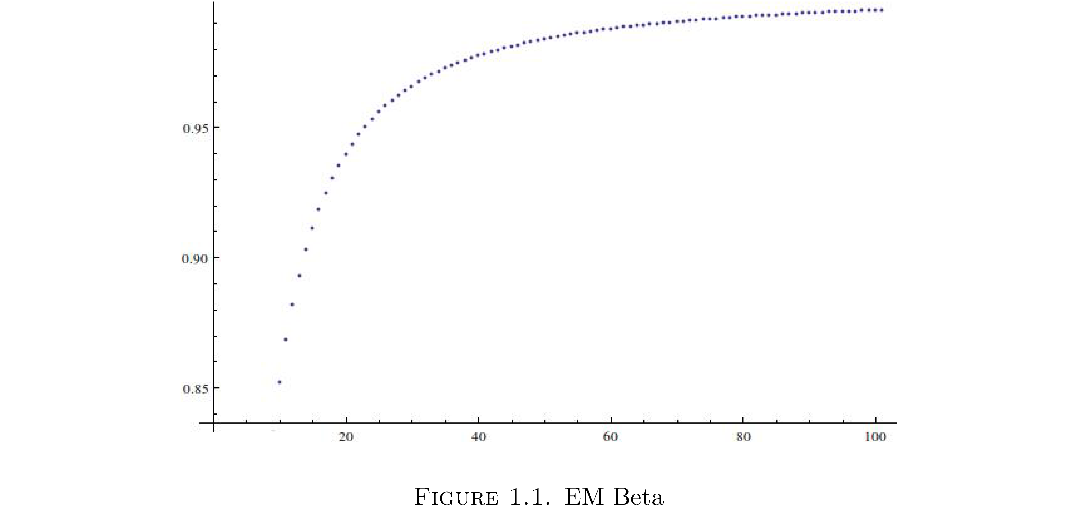
So they converge but to \(1\neq2/3\). Why did I present this algorithm first? Standard EM is slightly more complicated and much less intuitive but legend has it that it was in fact conceived in this way first and then manipulated to get convergence.

Expectation Maximization for Real

Recall that the whole point of this procedure is to actually maximize the likelihood for \(\mathbf{Y}\). This is equivalent to maximizing the log-likelihood for \(\mathbf{Y}\)

\[l\left(\boldsymbol{\theta};\mathbf{y}\right)=\log L\left(\boldsymbol{\theta};\mathbf{y}\right)=\log f_{\mathbf{Y}}\left(\mathbf{y};\boldsymbol{\theta}\right)\]

The ansatz here is the same: suppose there exists another random, unobserved, vector \(\mathbf{X}\) such that were \(\mathbf{X}\) in fact observed, maximizing the joint log-likelihood for \(\mathbf{X}\) and \(\mathbf{Y}\)

\[l\left(\boldsymbol{\theta};\mathbf{x},\mathbf{y}\right)=\log L\left(\boldsymbol{\theta};\mathbf{x},\mathbf{y}\right)=\log f_{\mathbf{X},\mathbf{Y}}\left(\mathbf{x},\mathbf{y};\boldsymbol{\theta}\right)\]

is easier than the original problem. The ease of maximizing \(l\left(\boldsymbol{\theta};\mathbf{x},\mathbf{y}\right)\) over \(l\left(\boldsymbol{\theta};\mathbf{y}\right)\) isn’t immediately apparent but first using Bayes’ theorem we see that

\[\begin{align} l\left(\boldsymbol{\theta};\mathbf{y}\right) & =\log f_{\mathbf{Y}}\left(\mathbf{y};\boldsymbol{\theta}\right)\\ & =\log\left(\frac{f_{\mathbf{X},\mathbf{Y}}\left(\mathbf{x},\mathbf{y};\boldsymbol{\theta}\right)}{f_{\mathbf{X}|\mathbf{Y}}\left(\mathbf{x}|\mathbf{y};\boldsymbol{\theta}\right)}\right)\\ & =\log\left(f_{\mathbf{X},\mathbf{Y}}\left(\mathbf{x},\mathbf{y};\boldsymbol{\theta}\right)\right)-\log\left(f_{\mathbf{X}|\mathbf{Y}}\left(\mathbf{x}|\mathbf{y};\boldsymbol{\theta}\right)\right)\label{eq:2.3}\end{align}\]

If we can easily maximize the first term in \(\eqref{eq:2.3}\), with respect to \(\boldsymbol{\theta}\) and the second term in \(\eqref{eq:2.3}\) doesn’t spoil things somehow, then we’ll indeed maximize \(l\left(\boldsymbol{\theta};\mathbf{y}\right)\). This seems like a workflow different from that of the beta algorithm⁵ but the analogy follows. Since \(\mathbf{X}\) is unobserved we face the same difficulty as in the beta algorithm: the terms in \(\eqref{eq:2.3}\) can’t be computed and must be estimated. We use the same estimator as before \(E\left[\cdot|\mathbf{y};\boldsymbol{\theta}^{\left(r\right)}\right]\)

\[l\left(\boldsymbol{\theta};\mathbf{y}\right)=E\left[\log\left(f_{\mathbf{X},\mathbf{Y}}\left(\mathbf{X},\mathbf{y};\boldsymbol{\theta}\right)\right)|\mathbf{y};\boldsymbol{\theta}^{\left(r\right)}\right]-E\left[\log\left(f_{\mathbf{X}|\mathbf{Y}}\left(\mathbf{X}|\mathbf{y};\boldsymbol{\theta}\right)\right)|\mathbf{y};\boldsymbol{\theta}^{\left(r\right)}\right]\label{eq:2.4}\]

Note some subtle things:

• \(\mathbf{x}\rightarrow\mathbf{X}\) because each of the terms on the right-hand side of \(\eqref{eq:2.4}\) are estimates of the random variable X as a function of observed data y.

• The expectations are again computed with respect to the conditional distribution of \(\mathbf{X}\) given Y for fixed (iterate) values of \(\boldsymbol{\theta}^{\left(r\right)}\), i.e. \(f_{\mathbf{X}|\mathbf{Y}}\left(\mathbf{x}|\mathbf{y};\boldsymbol{\theta}^{\left(r\right)}\right)\).

• The estimators, for which the expectations are computed, are functions of \(\boldsymbol{\theta}\).

• Equality is maintained because since \(l\left(\boldsymbol{\theta};\mathbf{y}\right)\) is independent of \(\mathbf{X}\)

  \[E\left[l\left(\boldsymbol{\theta};\mathbf{y}\right)|\mathbf{y};\boldsymbol{\theta}^{\left(r\right)}\right]=l\left(\boldsymbol{\theta};\mathbf{y}\right)\]

The algorithm then is

Expectation Algorithm. Given some observed data \(\mathbf{y}\), in order to perform the intractable maximization of \(L\left(\boldsymbol{\theta};\mathbf{y}\right)\), posit the existence of some latent \(\mathbf{X}\) such that \(L\left(\boldsymbol{\theta};\mathbf{x},\mathbf{y}\right)\) is easier. Set \(\boldsymbol{\theta}^{\left(0\right)}\) to be some initial guess for \(\boldsymbol{\theta}\) then

1. E-step: Compute \(E\left[\log\left(f_{\mathbf{X},\mathbf{Y}}\left(\mathbf{X},\mathbf{y};\boldsymbol{\theta}\right)\right)|\mathbf{y};\boldsymbol{\theta}^{\left(r\right)}\right]\)

   1. M-step: Set \(\boldsymbol{\theta}^{\left(r+1\right)}=\arg\max_{\boldsymbol{\theta}}E\left[\log\left(f_{\mathbf{X},\mathbf{Y}}\left(\mathbf{X},\mathbf{y};\boldsymbol{\theta}\right)\right)|\mathbf{y};\boldsymbol{\theta}^{\left(r\right)}\right]\)

   2. Go to step 1 unless \(\left|\boldsymbol{\theta}^{\left(r+1\right)}-\boldsymbol{\theta}^{\left(r\right)}\right|<\varepsilon\) for some \(\varepsilon\) of your choosing.

The only thing to remains is to prove that maximizing \(E\left[\log\left(f_{\mathbf{X},\mathbf{Y}}\left(\mathbf{X},\mathbf{y};\boldsymbol{\theta}\right)\right)|\mathbf{y};\boldsymbol{\theta}^{\left(r\right)}\right]\) is sufficient to maximize \(l\left(\boldsymbol{\theta};\mathbf{y}\right)\). I won’t but I’ll prove a thing on the way to that result, namely that \(l\left(\boldsymbol{\theta}^{\left(r\right)};\mathbf{y}\right)\geq l\left(\boldsymbol{\theta}^{\left(r-1\right)};\mathbf{y}\right)\) and since \(l\left(\boldsymbol{\theta};\mathbf{y}\right)\) is bounded above (it’s a density) the sequence of \(l\left(\boldsymbol{\theta}^{\left(r\right)};\mathbf{y}\right)\) must converge. The last hurdle would be proving that convergence of \(l\left(\boldsymbol{\theta}^{\left(r\right)};\mathbf{y}\right)\) implies the convergence of the iterates \(\boldsymbol{\theta}^{\left(r\right)}\) themselves[1].

Theorem (Monotonic EM Sequence): The sequence \(\left\{ \boldsymbol{\theta}^{\left(r\right)}\right\}\) satisfies \(l\left(\boldsymbol{\theta}^{\left(r+1\right)};\mathbf{y}\right)\geq l\left(\boldsymbol{\theta}^{\left(r\right)};\mathbf{y}\right)\).

Proof: Start with

\[l\left(\boldsymbol{\theta};\mathbf{y}\right)=\log\left(f_{\mathbf{X},\mathbf{Y}}\left(\mathbf{x},\mathbf{y};\boldsymbol{\theta}\right)\right)-\log\left(f_{\mathbf{X}|\mathbf{Y}}\left(\mathbf{x}|\mathbf{y};\boldsymbol{\theta}\right)\right)\]

Take conditional expectation with respect to \(\mathbf{X}|\mathbf{Y};\boldsymbol{\theta}^{\left(r\right)}\) of both sides

\[\begin{align} \int l\left(\boldsymbol{\theta};\mathbf{y}\right)f_{\mathbf{X}|\mathbf{Y}}\left(\mathbf{x}|\mathbf{y};\boldsymbol{\theta}^{\left(r\right)}\right)d\mathbf{x} & =\int\log\left(f_{\mathbf{X},\mathbf{Y}}\left(\mathbf{x},\mathbf{y};\boldsymbol{\theta}\right)\right)f_{\mathbf{X}|\mathbf{Y}}\left(\mathbf{x}|\mathbf{y};\boldsymbol{\theta}^{\left(r\right)}\right)d\mathbf{x}\\ & -\int\log\left(f_{\mathbf{X}|\mathbf{Y}}\left(\mathbf{x}|\mathbf{y};\boldsymbol{\theta}\right)\right)f_{\mathbf{X}|\mathbf{Y}}\left(\mathbf{x}|\mathbf{y};\boldsymbol{\theta}^{\left(r\right)}\right)d\mathbf{x}\end{align}\]

Since \(l\left(\boldsymbol{\theta};\mathbf{y}\right)\) is independent of \(\mathbf{x}\)

\[\begin{align} \int l\left(\boldsymbol{\theta};\mathbf{y}\right)f_{\mathbf{X}|\mathbf{Y}}\left(\mathbf{x}|\mathbf{y};\boldsymbol{\theta}^{\left(r\right)}\right)d\mathbf{x} & =l\left(\boldsymbol{\theta};\mathbf{y}\right)\int f_{\mathbf{X}|\mathbf{Y}}\left(\mathbf{x}|\mathbf{y};\boldsymbol{\theta}^{\left(r\right)}\right)d\mathbf{x}\\ & =l\left(\boldsymbol{\theta};\mathbf{y}\right)\end{align}\]

and so

\[\begin{align} l\left(\boldsymbol{\theta};\mathbf{y}\right) & =\int\log\left(f_{\mathbf{X},\mathbf{Y}}\left(\mathbf{x},\mathbf{y};\boldsymbol{\theta}\right)\right)f_{\mathbf{X}|\mathbf{Y}}\left(\mathbf{x}|\mathbf{y};\boldsymbol{\theta}^{\left(r\right)}\right)d\mathbf{x}\\ & -\int\log\left(f_{\mathbf{X}|\mathbf{Y}}\left(\mathbf{x}|\mathbf{y};\boldsymbol{\theta}\right)\right)f_{\mathbf{X}|\mathbf{Y}}\left(\mathbf{x}|\mathbf{y};\boldsymbol{\theta}^{\left(r\right)}\right)d\mathbf{x}\\ & =E\left[\log\left(f_{\mathbf{X},\mathbf{Y}}\left(\mathbf{X},\mathbf{y};\boldsymbol{\theta}\right)\right)|\mathbf{y};\boldsymbol{\theta}^{\left(r\right)}\right]-E\left[\log\left(f_{\mathbf{X}|\mathbf{Y}}\left(\mathbf{X}|\mathbf{y};\boldsymbol{\theta}\right)\right)|\mathbf{y};\boldsymbol{\theta}^{\left(r\right)}\right]\end{align}\]

Let

\[Q\left(\mathbf{\boldsymbol{\theta}},\boldsymbol{\theta}^{\left(r\right)}\right)=E\left[\log\left(f_{\mathbf{X},\mathbf{Y}}\left(\mathbf{X},\mathbf{y};\boldsymbol{\theta}\right)\right)|\mathbf{y};\boldsymbol{\theta}^{\left(r\right)}\right]\]

and \(K\left(\boldsymbol{\theta},\boldsymbol{\theta}^{\left(r\right)}\right)=E\left[\log\left(f_{\mathbf{X}|\mathbf{Y}}\left(\mathbf{X}|\mathbf{y};\boldsymbol{\theta}\right)\right)|\mathbf{y};\boldsymbol{\theta}^{\left(r\right)}\right]\). Then

\[l\left(\boldsymbol{\theta};\mathbf{y}\right)=Q\left(\mathbf{\boldsymbol{\theta}},\boldsymbol{\theta}^{\left(r\right)}\right)-K\left(\boldsymbol{\theta},\boldsymbol{\theta}^{\left(r\right)}\right)\]

If we can show that

\[\begin{align} Q\left(\boldsymbol{\theta}^{\left(r\right)},\boldsymbol{\theta}^{\left(r\right)}\right) & \leq Q\left(\boldsymbol{\theta}^{\left(r+1\right)},\boldsymbol{\theta}^{\left(r\right)}\right)\\ & \text{and}\\ K\left(\boldsymbol{\theta}^{\left(r\right)},\boldsymbol{\theta}^{\left(r\right)}\right) & \geq K\left(\boldsymbol{\theta}^{\left(r+1\right)},\boldsymbol{\theta}^{\left(r\right)}\right)\end{align}\]

then it will follow that \(l\left(\boldsymbol{\theta}^{\left(r+1\right)};\mathbf{y}\right)\geq l\left(\boldsymbol{\theta}^{\left(r\right)};\mathbf{y}\right)\). Well by definition of

\[\boldsymbol{\theta}^{\left(r+1\right)}=\arg\max_{\boldsymbol{\theta}}E\left[\log\left(f_{\mathbf{X},\mathbf{Y}}\left(\mathbf{X},\mathbf{y};\boldsymbol{\theta}\right)\right)|\mathbf{y};\boldsymbol{\theta}^{\left(r\right)}\right]=\arg\max_{\boldsymbol{\theta}}Q\left(\mathbf{\boldsymbol{\theta}},\boldsymbol{\theta}^{\left(r\right)}\right)\]

so

\[Q\left(\mathbf{\boldsymbol{\theta}},\boldsymbol{\theta}^{\left(r\right)}\right)\leq Q\left(\mathbf{\boldsymbol{\theta}},\arg\max_{\boldsymbol{\theta}}Q\left(\mathbf{\boldsymbol{\theta}},\boldsymbol{\theta}^{\left(r\right)}\right)\right)=Q\left(\mathbf{\boldsymbol{\theta}},\boldsymbol{\theta}^{\left(r+1\right)}\right)\]

To see that \(K\left(\boldsymbol{\theta}^{\left(r\right)},\boldsymbol{\theta}^{\left(r\right)}\right)\geq K\left(\boldsymbol{\theta}^{\left(r+1\right)},\boldsymbol{\theta}^{\left(r\right)}\right)\) inspect

\[\int\log\left(\frac{f_{\mathbf{X}|\mathbf{Y}}\left(\mathbf{x}|\mathbf{y};\boldsymbol{\theta}^{\left(r+1\right)}\right)}{f_{\mathbf{X}|\mathbf{Y}}\left(\mathbf{x}|\mathbf{y};\boldsymbol{\theta}^{\left(r\right)}\right)}\right)f_{\mathbf{X}|\mathbf{Y}}\left(\mathbf{x}|\mathbf{y};\boldsymbol{\theta}^{\left(r\right)}\right)d\mathbf{x}\]

On the one hand

\[\begin{align} \int\log\left(\frac{f_{\mathbf{X}|\mathbf{Y}}\left(\mathbf{x}|\mathbf{y};\boldsymbol{\theta}^{\left(r+1\right)}\right)}{f_{\mathbf{X}|\mathbf{Y}}\left(\mathbf{x}|\mathbf{y};\boldsymbol{\theta}^{\left(r\right)}\right)}\right)f_{\mathbf{X}|\mathbf{Y}}\left(\mathbf{x}|\mathbf{y};\boldsymbol{\theta}^{\left(r\right)}\right)d\mathbf{x} & =\int\log\left(f_{\mathbf{X}|\mathbf{Y}}\left(\mathbf{x}|\mathbf{y};\boldsymbol{\theta}^{\left(r+1\right)}\right)\right)f_{\mathbf{X}|\mathbf{Y}}\left(\mathbf{x}|\mathbf{y};\boldsymbol{\theta}^{\left(r\right)}\right)d\mathbf{x}\\ & -\int\log\left(f_{\mathbf{X}|\mathbf{Y}}\left(\mathbf{x}|\mathbf{y};\boldsymbol{\theta}^{\left(r\right)}\right)\right)f_{\mathbf{X}|\mathbf{Y}}\left(\mathbf{x}|\mathbf{y};\boldsymbol{\theta}^{\left(r\right)}\right)d\mathbf{x}\\ & =K\left(\boldsymbol{\theta}^{\left(r+1\right)},\boldsymbol{\theta}^{\left(r\right)}\right)-K\left(\boldsymbol{\theta}^{\left(r\right)},\boldsymbol{\theta}^{\left(r\right)}\right)\end{align}\]

on the other hand, by Jensen’s⁶ inequality⁷

\[\begin{align} \int\log\left(\frac{f_{\mathbf{X}|\mathbf{Y}}\left(\mathbf{x}|\mathbf{y};\boldsymbol{\theta}^{\left(r+1\right)}\right)}{f_{\mathbf{X}|\mathbf{Y}}\left(\mathbf{x}|\mathbf{y};\boldsymbol{\theta}^{\left(r\right)}\right)}\right)f_{\mathbf{X}|\mathbf{Y}}\left(\mathbf{x}|\mathbf{y};\boldsymbol{\theta}^{\left(r\right)}\right)d\mathbf{x} & \leq\log\left[\int\left(\frac{f_{\mathbf{X}|\mathbf{Y}}\left(\mathbf{x}|\mathbf{y};\boldsymbol{\theta}^{\left(r+1\right)}\right)}{f_{\mathbf{X}|\mathbf{Y}}\left(\mathbf{x}|\mathbf{y};\boldsymbol{\theta}^{\left(r\right)}\right)}\right)f_{\mathbf{X}|\mathbf{Y}}\left(\mathbf{x}|\mathbf{y};\boldsymbol{\theta}^{\left(r\right)}\right)d\mathbf{x}\right]\\ & =\log\left[\int f_{\mathbf{X}|\mathbf{Y}}\left(\mathbf{x}|\mathbf{y};\boldsymbol{\theta}^{\left(r+1\right)}\right)d\mathbf{x}\right]\\ & =0\end{align}\]

Hence

\[K\left(\boldsymbol{\theta}^{\left(r+1\right)},\boldsymbol{\theta}^{\left(r\right)}\right)-K\left(\boldsymbol{\theta}^{\left(r\right)},\boldsymbol{\theta}^{\left(r\right)}\right)\leq0\]

which completes the proof.

Applications

Gaussian Mixture Models

EM works really well for mixture models, e.g. \(\mathbf{Y}_{i}\) is distributed iid such that

\[f_{\mathbf{Y}_{1}}\left(\mathbf{y}_{1}\right)=\sum_{j=1}^{m}\alpha_{j}g_{j}\left(\mathbf{y}_{1};\boldsymbol{\theta}_{j}\right)\]

where \(g_{j}\) are (in general multivariate) densities with parameter vectors \(\boldsymbol{\theta}_{j}\) (in general, distinct for distinct \(j\)) and \(\sum_{j}\alpha_{j}=1\). If \(g_{j}\sim\text{n}\left(\mu_{j},\sigma_{j}^{2}\right)\) then the mixture model is called a Gaussian mixture model (GMM). Naively if you wanted to find the MLEs you would maximize

\[L\left(\left(\mathbf{y}_{1},\dots,\mathbf{y}_{n}\right);\boldsymbol{\theta}\right)=\prod_{i=1}^{n}f_{\mathbf{Y}_{i}}\left(\mathbf{y}_{i};\boldsymbol{\theta}\right)=\prod_{i=1}^{n}\sum_{j=1}^{m}\alpha_{j}g_{j}\left(\mathbf{y}_{i};\boldsymbol{\theta}_{j}\right)\]

Even taking the log won’t help you because of the interior sum. EM to the rescue! Let \(\mathbf{X}=\left(X_{1},\dots,X_{n}\right)\) be the mixture components, i.e. each \(X_{i}\) is a categorical random variable that indicates which component of the mixture density produced the correspondent \(\mathbf{Y}_{i}\)

\[\begin{align} P\left(X_{i}=j\right) & =\begin{cases} \alpha_{0} & \text{ if }x_{i}=0\\ \alpha_{1} & \text{ if }x_{i}=1\\ \vdots\\ \alpha_{m} & \text{ if }x_{i}=m \end{cases}\end{align}\]

Hence

\[\begin{align} P\left(X_{i}=j\right) & = & a_{j}\end{align}\]

And the \(\mathbf{Y}_{i}\mid X_{i}\) takes the form

\[f_{\mathbf{Y}_{i}|X_{i}}\left(\mathbf{y}_{i}|x_{i}=j;\boldsymbol{\theta}\right)=g_{j}\left(\mathbf{y}_{i};\boldsymbol{\theta}_{j}\right)\]

The \(x_{i}\) in \(g_{x_{i}}\left(\mathbf{y}_{i};\boldsymbol{\theta}_{x_{i}}\right)\) “picks” which mixture component the \(\mathbf{y}_{i}\) is generated by. Then the log-likelihood becomes

\[\begin{align} l\left(\left(x_{1},\dots,x_{n}\right),\left(\mathbf{y}_{1},\dots,\mathbf{y}_{n}\right);\boldsymbol{\theta}\right) & =\log\left[\prod_{i=1}^{n}f_{X_{i},\mathbf{Y}_{i}}\left(x_{i},\mathbf{y}_{i};\boldsymbol{\theta}\right)\right]\\ & =\log\left[\prod_{i=1}^{n}\left[f_{\mathbf{Y}_{i}|X_{i}}\left(\mathbf{y}_{i}|x_{i};\boldsymbol{\theta}\right)P\left(X_{i}=j\right)\right]\right]\\ & =\log\left[\prod_{i=1}^{n}\left[g_{j}\left(\mathbf{y}_{i};\boldsymbol{\theta}_{j}\right)\alpha_{j}\right]\right]\\ & =\sum_{i=1}^{n}\log\left(g_{j}\left(\mathbf{y}_{i};\boldsymbol{\theta}_{j}\right)\alpha_{j}\right)\\ & =\sum_{i=1}^{n}\left[\log\alpha_{j}+\log\left(g_{j}\left(\mathbf{y}_{i};\boldsymbol{\theta}_{j}\right)\right)\right]\end{align}\]

There are a lot of indices and subscripts and superscripts to keep track of: \(\boldsymbol{\theta}\) is all of the parameters of all of the mixture components, \(\mathbf{y}_{i}\) are observed samples (\(n\) of them), the \(X_{i}\) are the unobserved data (the mixture components), the \(\boldsymbol{\theta}_{j}\) are the parameters of the \(j\)th mixture density, and the \(\alpha_{j}\) are the mixture coefficients (i.e. in what proportion the \(j\)th density contributes). Much as we did for Example 1 we need to compute \(f_{X_{i}|\mathbf{Y}_{i}}\left(x_{i}|\mathbf{y}_{i};\boldsymbol{\theta}^{\left(r\right)}\right)=P\left(X_{i}=j|\mathbf{y}_{i};\boldsymbol{\theta}^{\left(r\right)}\right)\) in order to compute the conditional expectations

\[\begin{align} P\left(X_{i}=j|\mathbf{y}_{i};\boldsymbol{\theta}^{\left(r\right)}\right) & =\frac{f_{X_{i},\mathbf{Y}_{i}}\left(j,\mathbf{y}_{i};\boldsymbol{\theta}^{\left(r\right)}\right)}{f_{\mathbf{Y}_{i}}\left(\mathbf{y}_{i};\theta\right)}\\ & =\frac{g_{j}\left(\mathbf{y}_{i};\boldsymbol{\theta}_{j}^{\left(r\right)}\right)\alpha_{j}^{\left(r\right)}}{\sum_{k=1}^{m}\left(g_{k}\left(\mathbf{y}_{i};\boldsymbol{\theta}_{k}^{\left(r\right)}\right)\alpha_{k}^{\left(r\right)}\right)}\end{align}\]

So again \(X_{i}\mid\mathbf{Y}_{i}\) is categorical random variable. By i.i.d

\[P\left(\left(X_{1}=j_{1},\dots,X_{n}=j_{n}\right)|\left(\mathbf{y}_{1},\dots,\mathbf{y}_{n}\right);\boldsymbol{\theta}^{\left(r\right)}\right)=\prod_{i=1}^{n}\frac{g_{j}\left(\mathbf{y}_{i};\boldsymbol{\theta}_{j}^{\left(r\right)}\right)\alpha_{j_{i}}^{\left(r\right)}}{\sum_{k=1}^{m}\left(g_{k}\left(\mathbf{y}_{i};\boldsymbol{\theta}_{k}^{\left(r\right)}\right)\alpha_{k}^{\left(r\right)}\right)}\]

Now we just need to take the expectation of the log-likelihood against this conditional density

\[\begin{align} E\left[l\left(\left(X_{1},\dots,X_{n}\right),\left(\mathbf{y}_{1},\dots,\mathbf{y}_{n}\right);\boldsymbol{\theta}\right)|\left(\mathbf{y}_{1},\dots,\mathbf{y}_{n}\right);\boldsymbol{\theta}^{\left(r\right)}\right]=\\ \sum_{j_{1}=1}^{m}\sum_{j_{2}=1}^{m}\cdots\sum_{j_{n}=1}^{m}\left(\left[\sum_{k=1}^{n}\left\{ \log\alpha_{j_{k}}+\log\left[g_{j_{k}}\left(\mathbf{y}_{k};\boldsymbol{\theta}_{j_{k}}\right)\right]\right\} \right]\prod_{i=1}^{n}\frac{g_{j}\left(\mathbf{y}_{i};\boldsymbol{\theta}_{j}^{\left(r\right)}\right)\alpha_{j}^{\left(r\right)}}{\sum_{k=1}^{m}\left(g_{k}\left(\mathbf{y}_{i};\boldsymbol{\theta}_{k}^{\left(r\right)}\right)\alpha_{k}^{\left(r\right)}\right)}\right)\end{align}\]

Pretty ugly right? Suffice it to say you’re not actually taking this expectation. So let

\[\gamma_{ij}^{\left(r\right)}\coloneqq P\left(X_{i}=j|\mathbf{y}_{i};\boldsymbol{\theta}^{\left(r\right)}\right)=\frac{g_{j}\left(\mathbf{y}_{i};\boldsymbol{\theta}_{j}^{\left(r\right)}\right)\alpha_{j}^{\left(r\right)}}{\sum_{k=1}^{m}\left(g_{k}\left(\mathbf{y}_{i};\boldsymbol{\theta}_{k}^{\left(r\right)}\right)\alpha_{k}^{\left(r\right)}\right)}\]

and a helpful lemma:

Lemma 1: For i.i.d incomplete samples \(Y_{i}\), with completions \(X_{i}\)

\[E\left[l\left(\left(X_{1},\dots,X_{n}\right),\left(\mathbf{y}_{1},\dots,\mathbf{y}_{n}\right);\boldsymbol{\theta}\right)|\left(\mathbf{y}_{1},\dots,\mathbf{y}_{n}\right);\boldsymbol{\theta}^{\left(r\right)}\right]=\sum_{i=1}^{n}E\left[l\left(X_{i}|\mathbf{y}_{i};\boldsymbol{\theta}\right)|\mathbf{y}_{i};\boldsymbol{\theta}^{\left(r\right)}\right]\]

where \(\mathbf{y}_{i}\) is the ith sample.

Proof: By i.i.d

\[\begin{align} E\left[l\left(\left(X_{1},\dots,X_{n}\right),\left(\mathbf{y}_{1},\dots,\mathbf{y}_{n}\right);\boldsymbol{\theta}\right)|\left(\mathbf{y}_{1},\dots,\mathbf{y}_{n}\right);\boldsymbol{\theta}^{\left(r\right)}\right] & =\\ E\left[\log\left[\prod_{i=1}^{n}f\left(X_{i}|\left(\mathbf{y}_{1},\dots,\mathbf{y}_{n}\right);\boldsymbol{\theta}\right)\right]|\left(\mathbf{y}_{1},\dots,\mathbf{y}_{n}\right);\boldsymbol{\theta}^{\left(r\right)}\right] & =\\ E\left[\sum_{i=1}^{n}\log\left[f\left(X_{i}|\left(\mathbf{y}_{1},\dots,\mathbf{y}_{n}\right);\boldsymbol{\theta}\right)\right]|\left(\mathbf{y}_{1},\dots,\mathbf{y}_{n}\right);\boldsymbol{\theta}^{\left(r\right)}\right] & =\left(\text{ since }X_{i}\perp X_{j}\text{ for }i\neq j\right)\\ \sum_{i=1}^{n}E\left[\log\left[f\left(X_{i}|\left(\mathbf{y}_{1},\dots,\mathbf{y}_{n}\right);\boldsymbol{\theta}\right)\right]|\left(\mathbf{y}_{1},\dots,\mathbf{y}_{n}\right);\boldsymbol{\theta}^{\left(r\right)}\right] & =\left(\text{ since }P\left(X_{i}=x_{i}|\left(\mathbf{Y}_{1},\dots,\mathbf{Y}_{n}\right)\right)=P\left(X_{i}=x_{i}|\mathbf{Y}_{i}\right)\right)\\ \sum_{i=1}^{n}E\left[\log\left[f\left(X_{i}|\mathbf{y}_{i};\boldsymbol{\theta}\right)\right]|\mathbf{y}_{i};\boldsymbol{\theta}^{\left(r\right)}\right] & =\\ \sum_{i=1}^{n}E\left[l\left(X_{i}|\mathbf{y}_{i};\boldsymbol{\theta}\right)|\mathbf{y}_{i};\boldsymbol{\theta}^{\left(r\right)}\right]\end{align}\]

Therefore we only need to compute \(E\left[l\left(X_{i}|\mathbf{y}_{i};\boldsymbol{\theta}\right)|\mathbf{y}_{i};\boldsymbol{\theta}^{\left(r\right)}\right]\) to perform the E-step. Let \(j_{i}\rightarrow j\) for convenience and \(\left(\mu_{j},\Sigma_{j}\right)\) be the parameters for the \(j\)th Gaussian. Actually let’s take the 1 dimensional Gaussian case⁸ so \(\left(\mu_{j},\Sigma_{j}\right)=\left(\mu_{j},\sigma_{j}^{2}\right)\) and \(\mathbf{y}_{i}\rightarrow y_{i}\).

\[\begin{align} E\left[l\left(X_{i}|y_{i};\boldsymbol{\theta}\right)|y_{i};\boldsymbol{\theta}^{\left(r\right)}\right] & =\sum_{j=1}^{m}\left(\left[\log\alpha_{j}+\log\left(g_{j}\left(y_{i};\boldsymbol{\theta}_{j}\right)\right)\right]\gamma_{ij}^{\left(r\right)}\right)\\ & =\sum_{j=1}^{m}\left(\left[\log\alpha_{j}+\left(-\frac{1}{2}\left(\log\left(\sigma_{j}^{2}\right)+\log\left(2\pi\right)\right)-\frac{1}{2\sigma_{j}^{2}}\left(y_{i}-\mu_{j}\right)^{2}\right)\right]\gamma_{ij}^{\left(r\right)}\right)\end{align}\]

Then

\[\begin{align} E\left[l\left(\left(X_{1},\dots,X_{n}\right)|\left(y_{1},\dots,y_{n}\right);\boldsymbol{\theta}\right)|\left(y_{1},\dots,y_{n}\right);\boldsymbol{\theta}^{\left(r\right)}\right] & =\\ \sum_{i=1}^{n}\sum_{j=1}^{m}\left(\left[\log\alpha_{j}+\log\left(g_{j}\left(y_{i};\boldsymbol{\theta}_{j}\right)\right)\right]\gamma_{ij}^{\left(r\right)}\right) & =\\ \sum_{i=1}^{n}\sum_{j=1}^{m}\left(\left[\log\alpha_{j}+\left(-\frac{1}{2}\left(\log\left(\sigma_{j}^{2}\right)+\log\left(2\pi\right)\right)-\frac{1}{2\sigma_{j}^{2}}\left(y_{i}-\mu_{j}\right)^{2}\right)\right]\gamma_{ij}^{\left(r\right)}\right)\end{align}\]

Define

\[n_{j}^{\left(r\right)}=\sum_{i=1}^{n}\gamma_{ij}^{\left(r\right)}=\sum_{i=1}^{n}P\left(X_{i}=j|\mathbf{y}_{i};\boldsymbol{\theta}^{\left(r\right)}\right)\]

This is something like the portion of the samples that were generated by the \(j\)th component of the density⁹. The expectation becomes

\[\begin{align} E\left[l\left(\left(X_{1},\dots,X_{n}\right)|\left(y_{1},\dots,y_{n}\right);\boldsymbol{\theta}\right)|\left(y_{1},\dots,y_{n}\right);\boldsymbol{\theta}^{\left(r\right)}\right] & =\\ \sum_{i=1}^{n}\sum_{j=1}^{m}\left(\left[\log\alpha_{j}+\left(-\frac{1}{2}\left(\log\left(\sigma_{j}^{2}\right)+\log\left(2\pi\right)\right)-\frac{1}{2\sigma_{j}^{2}}\left(y_{i}-\mu_{j}\right)^{2}\right)\right]\gamma_{ij}^{\left(r\right)}\right) & =\\ \sum_{i=1}^{n}\sum_{j=1}^{m}\log\alpha_{j}\gamma_{ij}^{\left(r\right)}-\sum_{i=1}^{n}\sum_{j=1}^{m}\frac{1}{2}\left(\log\left(\sigma_{j}^{2}\right)+\log\left(2\pi\right)\right)\gamma_{ij}^{\left(r\right)}-\sum_{i=1}^{n}\sum_{j=1}^{m}\frac{1}{2\sigma_{j}^{2}}\left(y_{i}-\mu_{j}\right)^{2}\gamma_{ij}^{\left(r\right)} & =\\ \sum_{j=1}^{m}n_{j}^{\left(r\right)}\log\alpha_{j}-\frac{1}{2}\sum_{j=1}^{m}n_{j}^{\left(r\right)}\left(\log\left(\sigma_{j}^{2}\right)+\log\left(2\pi\right)\right)-\frac{1}{2}\sum_{i=1}^{n}\sum_{j=1}^{m}\frac{\left(y_{i}-\mu_{j}\right)^{2}}{\sigma_{j}^{2}}\gamma_{ij}^{\left(r\right)}\end{align}\]

This is the expression that needs to be maximized with respect to \(\alpha_{j},\mu_{j},\sigma_{j}^{2}\)¹⁰. The fully specified maximization problem is

\[\begin{align} \max_{\alpha_{j},\mu_{j},\sigma_{j}^{2}} & E\left[l\left(\left(X_{1},\dots,X_{n}\right)|\left(y_{1},\dots,y_{n}\right);\boldsymbol{\theta}\right)|\left(y_{1},\dots,y_{n}\right);\boldsymbol{\theta}^{\left(r\right)}\right]\\ & \iff\\ \max_{\alpha_{j},\mu_{j},\sigma_{j}^{2}} & \sum_{j=1}^{m}n_{j}^{\left(r\right)}\log\alpha_{j}-\frac{1}{2}\sum_{j=1}^{m}n_{j}^{\left(r\right)}\left(\log\left(\sigma_{j}^{2}\right)+\log\left(2\pi\right)\right)-\frac{1}{2}\sum_{i=1}^{n}\sum_{j=1}^{m}\frac{\left(y_{i}-\mu_{j}\right)^{2}}{\sigma_{j}^{2}}\gamma_{ij}^{\left(r\right)}\\ \text{subject to} & \sum_{j=1}^{m}\alpha_{j}=1,\:\alpha_{j}\geq0\end{align}\]

This looks tough but because it’s a bunch of uncoupled (somewhat) terms summed together so it’s easier than the original log-likelihood

\[\log\left[\sum_{j=1}^{m}\alpha_{j}g_{j}\left(\mathbf{y}_{i};\boldsymbol{\theta}_{j}\right)\right]\]

The local maxima for \(\alpha_{j},\mu_{j},\sigma_{j}^{2}\) become the new iterates, ie. \(\alpha_{j}^{\left(r+1\right)},\mu_{j}^{\left(r+1\right)},\left(\sigma_{j}^{2}\right)^{\left(r+1\right)}\). To perform the constrained maximization (only the \(\alpha_{j}\)) we use Lagrange multipliers; form the Lagrangian

\[\mathcal{L}\left(\boldsymbol{\alpha},\lambda\right)=\sum_{j=1}^{m}n_{j}^{\left(r\right)}\log\alpha_{j}+\lambda\left(\sum_{j=1}^{m}\alpha_{j}-1\right)\]

Then computing derivatives and setting to zero to find \(\alpha_{j}\)

\[\begin{align} \frac{\partial\mathcal{L}}{\partial\alpha_{j}} & = & \frac{n_{j}^{\left(r\right)}}{\alpha_{j}}+\lambda\end{align}\]

Therefore the critical¹¹ \(\alpha_{j}\) satisfy

\[\alpha_{j}=-\frac{n_{j}^{\left(r\right)}}{\lambda}\]

To eliminate \(\lambda\) use the equality constraint, i.e. \(\sum_{j=1}^{m}\alpha_{j}=1\) implies \(\lambda=-\sum_{j=1}^{m}n_{j}^{\left(r\right)}\) and hence

\[\alpha_{j}^{\left(r+1\right)}=\frac{n_{j}^{\left(r\right)}}{\sum_{j=1}^{m}n_{j}^{\left(r\right)}}=\frac{n_{j}^{\left(r\right)}}{n}\]

So \(\alpha_{j}^{\left(r+1\right)}\) is just the current best estimate for how many of the samples were generated by the \(j\)th component of the mixture density¹². To compute the updates \(\mu_{j}^{\left(r+1\right)}\) we just need to do the standard maximization of \(E\left[l\left(\left(X_{1},\dots,X_{n}\right)|\left(y_{1},\dots,y_{n}\right);\boldsymbol{\theta}\right)|\left(y_{1},\dots,y_{n}\right);\boldsymbol{\theta}^{\left(r\right)}\right]\) since the \(\mu_{j}\) are unconstrained. Therefore

\[\frac{\partial}{\partial\mu_{j}}E\left[l\left(\left(X_{1},\dots,X_{n}\right)|\left(y_{1},\dots,y_{n}\right);\boldsymbol{\theta}\right)|\left(y_{1},\dots,y_{n}\right);\boldsymbol{\theta}^{\left(r\right)}\right]=\sum_{i=1}^{n}\frac{\left(y_{i}-\mu_{j}\right)}{\sigma_{j}^{2}}\gamma_{ij}^{\left(r\right)}=0\]

Note the sum of \(j\) disappears because only the \(j\)th term is non-zero. Then simplifying further

\[\begin{align} \sum_{i=1}^{n}\frac{\left(y_{i}-\mu_{j}\right)}{\sigma_{j}^{2}}\gamma_{ij}^{\left(r\right)} & =\frac{1}{\sigma_{j}^{2}}\left(\sum_{i=1}^{n}\gamma_{ij}^{\left(r\right)}y_{i}-\mu_{j}\sum_{i=1}\gamma_{ij}^{\left(r\right)}\right)\\ & =\frac{1}{\sigma_{j}^{2}}\left(\sum_{i=1}^{n}\gamma_{ij}^{\left(r\right)}y_{i}-\mu_{j}n_{j}^{\left(r\right)}\right)=0\\ & \Rightarrow\\ \mu_{j}^{\left(r+1\right)} & =\frac{1}{n_{j}^{\left(r\right)}}\sum_{i=1}^{n}\gamma_{ij}^{\left(r\right)}y_{i}\end{align}\]

Finally doing the same kind of thing for \(\left(\sigma_{j}^{2}\right)^{\left(r+1\right)}\)

\[\frac{\partial}{\partial\sigma_{j}^{2}}E\left[l\left(\left(X_{1},\dots,X_{n}\right)|\left(y_{1},\dots,y_{n}\right);\boldsymbol{\theta}\right)|\left(y_{1},\dots,y_{n}\right);\boldsymbol{\theta}^{\left(r\right)}\right]=-\frac{1}{2}\frac{n_{j}^{\left(r\right)}}{\sigma_{j}^{2}}+\frac{1}{2}\sum_{i=1}^{n}\frac{\left(y_{i}-\mu_{j}^{\left(r+1\right)}\right)^{2}}{\left(\sigma_{j}^{2}\right)^{2}}\gamma_{ij}^{\left(r\right)}=0\]

where \(\mu_{j}\) now gets a superscript because it’s already been updated. Hence

\[\left(\sigma_{j}^{2}\right)^{\left(r+1\right)}=\frac{1}{n_{j}^{\left(r+1\right)}}\sum_{i=1}^{n}\left(y_{i}-\mu_{j}^{\left(r+1\right)}\right)^{2}\gamma_{ij}^{\left(r\right)}\]

In summary the update equations for a univariate GMM

\[\begin{align} \alpha_{j}^{\left(r+1\right)} & =\frac{n_{j}^{\left(r\right)}}{n}\\ \mu_{j}^{\left(r+1\right)} & =\frac{1}{n_{j}^{\left(r\right)}}\sum_{i=1}^{n}\gamma_{ij}^{\left(r\right)}y_{i}\\ \left(\sigma_{j}^{2}\right)^{\left(r+1\right)} & =\frac{1}{n_{j}^{\left(r+1\right)}}\sum_{i=1}^{n}\left(y_{i}-\mu_{j}^{\left(r+1\right)}\right)^{2}\gamma_{ij}^{\left(r\right)}\end{align}\]

where

\[\begin{align} \gamma_{ij}^{\left(r\right)} & =\frac{g_{j}\left(\mathbf{y}_{i};\boldsymbol{\theta}_{j}^{\left(r\right)}\right)\alpha_{j}^{\left(r\right)}}{\sum_{k=1}^{m}\left(g_{k}\left(\mathbf{y}_{i};\boldsymbol{\theta}_{k}^{\left(r\right)}\right)\alpha_{k}^{\left(r\right)}\right)}\\ n_{j}^{\left(r\right)} & =\sum_{i}\gamma_{ij}^{\left(r\right)}\end{align}\]

For multivariate GMM the only difference is \(\sigma_{j}^{2}\rightarrow\Sigma_{j}\) and so you need to use matrix derivatives. Consult [2] for the full derivation

\[\Sigma_{j}^{\left(r+1\right)}=\frac{1}{n_{j}^{\left(r+1\right)}}\sum_{i=1}^{n}\left(\mathbf{y}_{i}-\boldsymbol{\mu}_{j}^{\left(r+1\right)}\right)\left(\mathbf{y}_{i}-\boldsymbol{\mu}_{j}^{\left(r+1\right)}\right)^{T}\gamma_{ij}^{\left(r\right)}\]

References

Footnotes