
Girsanov theorem intuition
This post follows this video and this video and covers the intuition for change of measure for a stochastic process and stochastic differential equations.
Stochastic processes
Consider a collection Normal random variables
\[X_0, X_1, X_2, \dots, X_n\]where the indices can be taken to correspond to discrete times
\[t_0 < t_1 < t_2 < \cdots < t_n\]This is a finite dimensional stochastic process. Assume that $P(X_0 = 0) = 1$ and that increments $\Delta X_i := X_{i+1} - X_i$ are independent and distributed Normal
\[\Delta X_i \sim N(0, \Delta t_i)\]where $\Delta t_i := t_{i+1} - t_i$.
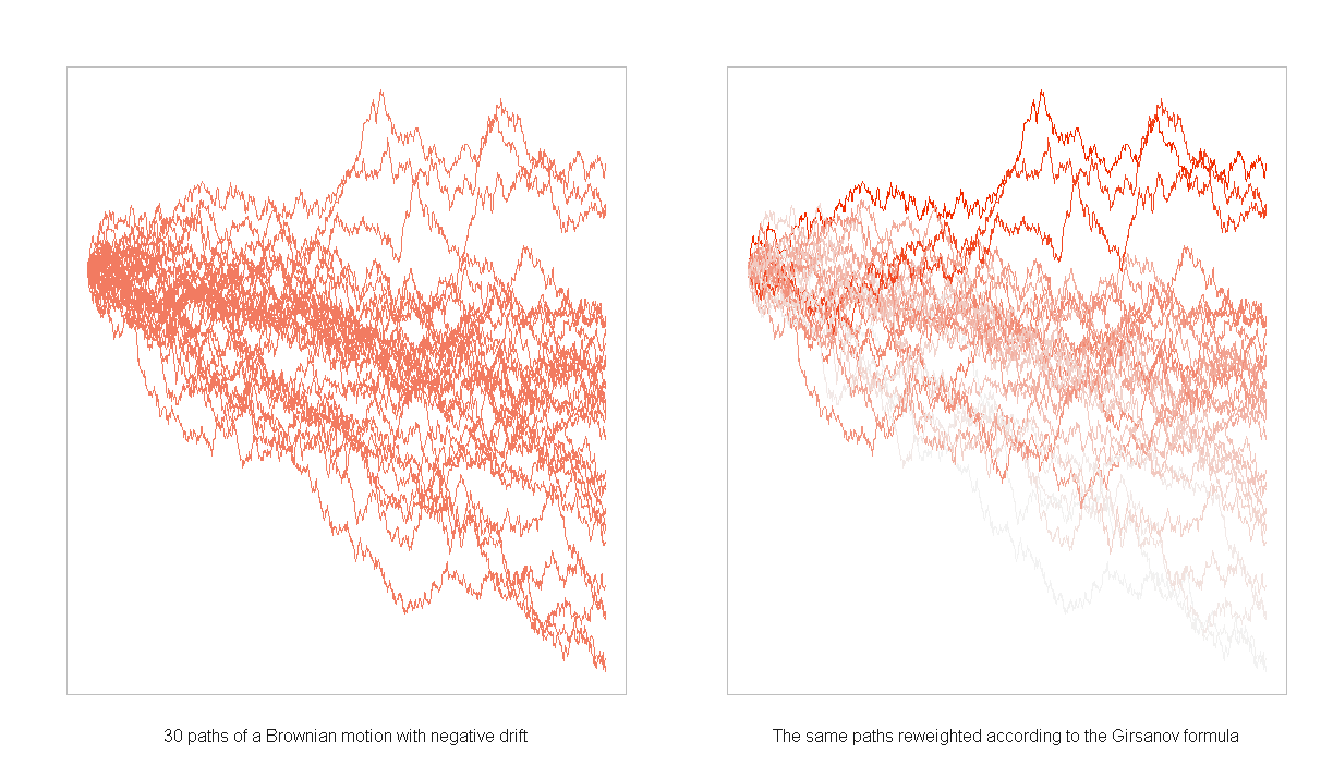
A mechanical procedure for generating $X_i$ is to start at zero, draw an increment some time $\Delta t$ later, add it to the previous total sum, and repeat. Here’s what several such trajectories (sample paths) look like

The unconditional distribution for $X_n$ is
\[X_n := \sum_{i=1}^n \Delta X_i \sim N\left(0, t_n\right)\]The conditional distribution of $X_i$ given $X_{i-1}$, i.e. given its previous value, is
\[\begin{aligned} X_i | (X_{i-1} = x_{i-1}) &\sim N(x_{i-1}, \Delta t) \\ & \iff \\ p(x_i - x_{i-1} | x_{i-1}) &= \frac{1}{\sqrt{2\pi \Delta t}} e^ { -\frac{1}{2\Delta t} \left( x_i - x_{i-1} \right)^2 } \end{aligned}\]where $\Delta t$ is a fixed time increment.
We now ask what the probability of the event $A$ that each of the $X_i$ being within a range, i.e.
\[P(A) = P\left( \alpha_1 \leq X_1 \leq \beta_1, \alpha_2 \leq X_2 \leq \beta_2,\dots,\alpha_n \leq X_n \leq \beta_n \right)\]Since the conditional distributions are independent we can write this as
\[\begin{aligned} P(A) &= \int\limits_{\alpha_1}^{\beta_1}\int\limits_{\alpha_2}^{\beta_2}\cdots\int\limits_{\alpha_n}^{\beta_n} p(x_1) p(x_2 - x_1 | x_1) \cdots p(x_n - x_{n-1} | x_{n-1}) dx_1 dx_2 \cdots dx_n \\ &= \frac{1}{(2\pi \Delta t)^{n/2}}\int\limits_{\alpha_1}^{\beta_1}\int\limits_{\alpha_2}^{\beta_2}\cdots\int\limits_{\alpha_n}^{\beta_n} e^ { -\frac{1}{2\Delta t} \sum_{i=1}^{n} (x_i - x_{i-1})^2} dx_1 dx_2 \cdots dx_n \end{aligned}\]Now we change the measure on each random variable by shifting the intervals of each integral proportional to time
\[P\left(\alpha_1 -\mu_1 \Delta t \leq X_1 \leq \beta_1 - \mu_1 \Delta t, \dots, \alpha_n -\sum_{i=1}^n \mu_i \Delta t \leq X_n \leq \beta -\sum_{i=1}^n \mu_i \Delta t\right)\]Making the substitution into the integral
\[\begin{aligned} P(A-\mu) &= \int\limits_{ \alpha_1 -\mu_1 \Delta t}^{\beta_1 -\mu_1 \Delta t}\cdots\int\limits_{ \alpha_n -\sum_{i=1}^n \mu_i \Delta t}^{\beta_n -\sum_{i=1}^n\mu_i \Delta t} p(x_1) \cdots p(x_n - x_{n-1} | x_{n-1}) dx_1 dx_2 \cdots dx_n \end{aligned}\]Making the change of variables to restore the original limits of integration is similar to the 1D case. We demonstrate for the $n=2$ case
\[\begin{aligned} &=\frac{1}{2\pi \Delta t} \int\limits_{ \alpha_1 -\mu_1 \Delta t}^{\beta_1 -\mu_1 \Delta t}\int\limits_{ \alpha_2 - (\mu_1 + \mu_2)\Delta t}^{ \beta_2 - (\mu_1 + \mu_2)\Delta t} e^ { -\frac{1}{2\Delta t} (x_1-x_0)^2} e^{-\frac{1}{2\Delta t}(x_2-x_1)^2 } dx_1 dx_2 \end{aligned}\]Then $y_1 = x_1 + \mu_1 \Delta t$ implies
\[\begin{aligned} &=\frac{1}{2\pi \Delta t} \int\limits_{ \alpha_1 }^{\beta_1 }\int\limits_{ \alpha_2 - (\mu_1 + \mu_2)\Delta t}^{ \beta_2 - (\mu_1 + \mu_2)\Delta t} e^{ -\frac{1}{2\Delta t} (y_1-x_0-\mu_1 \Delta t)^2}e^{ -\frac{1}{2\Delta t}(x_2-y_1+\mu_1\Delta t)^2 } dy_1 dx_2 \end{aligned}\]and $y_2 = x_2 + (\mu_1 + \mu_2) \Delta t$ implies
\[\begin{aligned} &=\frac{1}{2\pi \Delta t} \int\limits_{ \alpha_1 }^{\beta_1 }\int\limits_{ \alpha_2 }^{ \beta_2 } e^{ -\frac{1}{2\Delta t} (y_1-x_0-\mu_1 \Delta t)^2 } e^{ -\frac{1}{2\Delta t}(y_2-(\mu_1+\mu_2)\Delta t-y_1+\mu_1\Delta t)^2 } dy_1 dy_2 \\ &=\frac{1}{2\pi \Delta t} \int\limits_{ \alpha_1 }^{\beta_1 }\int\limits_{ \alpha_2 }^{ \beta_2 } e^{ -\frac{1}{2\Delta t} (y_1-x_0-\mu_1 \Delta t)^2 } e^{ -\frac{1}{2\Delta t}(y_2-y_1-\mu_2 \Delta t)^2} dy_1 dy_2 \end{aligned}\]Then changing the dummy variable $y_i \rightarrow x_i$
\[\begin{aligned} &=\frac{1}{2\pi \Delta t} \int\limits_{ \alpha_1 }^{\beta_1 }\int\limits_{ \alpha_2 }^{ \beta_2 } e^{ -\frac{1}{2\Delta t} (x_1-x_0-\mu_1 \Delta t)^2 } e^{ -\frac{1}{2\Delta t}(x_2-x_1-\mu_2 \Delta t)^2 } dx_1 dx_2 \\ &=\frac{1}{2\pi \Delta t} \int\limits_{ \alpha_1 }^{\beta_1 }\int\limits_{ \alpha_2 }^{ \beta_2 } e^{ -\frac{1}{2\Delta t} \left(\sum_{i=1}^2 x_i - x_{i-1} -\mu_i \Delta t\right)^2} dx_1 dx_2 \end{aligned}\]Generalizing to $n$ time steps we get
\[\begin{aligned} P(A-\mu) &= \frac{1}{(2\pi \Delta t)^{n/2}} \int\limits_{ \alpha_1 }^{\beta_1 }\cdots\int\limits_{ \alpha_n }^{ \beta_n } e^{ -\frac{1}{2\Delta t} \left(\sum_{i=1}^n x_i - x_{i-1} -\mu_i \Delta t\right)^2} dx_1 \cdots dx_n \end{aligned}\]Now expanding the square and splitting the exponential
\[\begin{aligned} P(A-\mu) &= \frac{1}{(2\pi \Delta t)^{n/2}} \int\limits_{ \alpha_1 }^{\beta_1 }\cdots\int\limits_{ \alpha_n }^{ \beta_n } e^{ -\frac{1}{2\Delta t} \left(\sum_{i=1}^n \Delta x_i \right)^2}e^{ \sum_{i=1}^n \mu_i \Delta x_i -\frac{1}{2}\mu_i^2 \Delta t} dx_1 \cdots dx_n \end{aligned}\]Defining
\[Z_n = e^{ \sum_{i=1}^n \mu_i \Delta X_i -\frac{1}{2}\mu_i^2 \Delta t}\]we have just as in the single variable case
\[\begin{aligned} P(A-\mu) &= \int\limits_A z_n dP(x) \\ &= Q(A) \\ \frac{dQ}{dP} &= z_n \\ E^Q \left[ h(X) \right] &= E^P \left[ Z(X) h(X) \right] \end{aligned}\]Under this new measure $Q$
\[X_n \sim N \left(\sum_{i=1}^n \mu_i \Delta t, t_n \right)\]Note the difference w.r.t. the distribution of $X_n$ under the original measure $P$ i.e. $X_n$ under the new measure is mean shifted by $\sum_{i=1}^n \mu_i \Delta t$. It follows that under the new measure $Q$
\[X_n - \sum_{i=1}^n \mu_i \Delta t \sim N\left(0, t_n\right)\]What’s happening here is that the process is being centering by the change of measure
Girsanov
If we squint at
\[Z_n = e^{ \sum_{i=1}^n \mu_i \Delta X_i -\frac{1}{2}\mu_i^2 \Delta t}\]the sum in the exponential looks like the sum approximation to the Ito integral
\[\int\limits_0^t \mu_s dB - \frac{1}{2} \int\limits_0^t \mu_s^2 ds\]where in the limit as $\Delta t \rightarrow 0$ the process $X_i$ becomes a continuous-time Brownian motion $B_t$.
The Girsanov theorem states that if $B_t$ is a Brownian motion under a measure $P$ then shifting the intervals of integration (changing the measure) by
\[\int\limits_0^t \mu_s ds\]produces another measure $Q$ defined in terms of the Radon-Nikodym derivative $Z_t$
\[\frac{dQ}{dP} := Z_t := e^{ \int_0^t \mu_s dB_s - \frac{1}{2} \int_0^t \mu_s^2 ds }\]and under this new measure $Q$
\[\tilde{B}_t := B_t - \int\limits_0^t \mu_s ds\]is a Brownian motion.
A simplified form of Girsanov is in the case that where $\mu_t \equiv \mu$ i.e. $\mu$ doesn’t depend on time
\[\begin{aligned} Z_t &= e^{\mu B_t - \tfrac{1}{2} \mu^2 t} \\ \tilde{B}_t &= B_t - \mu t \end{aligned}\]Stochastic differential equations
Consider a stochastic differential equation (SDE)
\[dX_t = \mu dt + \sigma dB_t\]Note that $\mu dt$ is the drift term (i.e. over time the mean of the process will move $\mu\times t$).
Factoring $dX_t$
\[dX_t = \sigma \left(\frac{\mu}{\sigma} dt + dB_t\right)\]If we can find a new measure such that the term in the parentheses if the differential of a Brownian motion
\[d \tilde{B}_t = \frac{\mu}{\sigma} dt + dB_t\]then $dX_t - \tfrac{\mu}{\sigma} dt$ will have zero drift under this measure.
Inspecting $d\tilde{B}_t$ we see that the relationship with $B_t$ must be (through integration of both sides)
\[\tilde{B}_t = \frac{\mu}{\sigma} t + B_t\]Now applying Girsanov we have
\[\frac{dQ}{dP} = e^{-\tfrac{\mu}{\sigma} B_t -\tfrac{1}{2} \left(\tfrac{\mu}{\sigma}\right)^2 t}\]and rearranging $dB_t$ we have, for $dX_t$
\[\begin{aligned} dX_t &= \sigma \left(\frac{\mu}{\sigma} dt + dB_t\right) \\ &= \sigma \left(\frac{\mu}{\sigma} dt + \left( d\tilde{B}_t - \frac{\mu}{\sigma} dt\right)\right) \\ &= \sigma d\tilde{B}_t \end{aligned}\]which is manifestly a zero drift process.