
Signal Processing
Signal processing is the science of decomposing and transforming signals (for various purposes e.g. study, compression, augmentation, etc).
Basics
A signal is simply a function $x = f(t)$ or $y = f(t)$. There’s nothing special about the independent variable being $t$ and the dependent variable being $x$ or $y$, it’s simply conventional in this area. Continuous time signals are the functions you’re used to, e.g. a straight line $y = kt + c$, where $t$ can take on any value in an interval $[a,b]$ or a union of intervals. Discrete time signals are those functions that are only defined at particular values of $t$, e.g. $t=1,2,\dots, 100$. It is convention that discrete time signals are written with square brackets, i.e. $x[t]$ and $y[t]$.
The typical case is that one is interested in a value that changes over time, something like pulse, or blood pressure, or the amplitude of a guitar string at some point on the string, etc. In these instances the use of $t$ as the independent variable is fitting since the value we’re interested is a function of time. In the case of pulse we would be studying a discrete time signal $x[t]$ (since we’re observing beats per minute at $t = 1,2,3,\dots$ minutes). In the cases of blood pressure and string amplitude we would be studying continuous time signals $x(t)$ and $y(t)$ (since we’re observing each signal at all time instances over some period).
Periodic signals
Periodic signals are signals that repeat (i.e. produce the same values after a period of some time).
The period of such a signal is how long it takes before it repeats, usually denoted $T$. The frequency $f$ is how many times the signal repeats in one unit of time (usually a second). For example if the period is $0.1$ seconds then the frequency is $1/0.1=10$. In general $f = 1/T$. When time is measured in physical units, i.e. seconds, frequency has unit $1/s = \text{Hz}$, named Hertz after Heinrich Hertz. So for the just prior example the signal would have a frequency of $10\text{Hz}$.
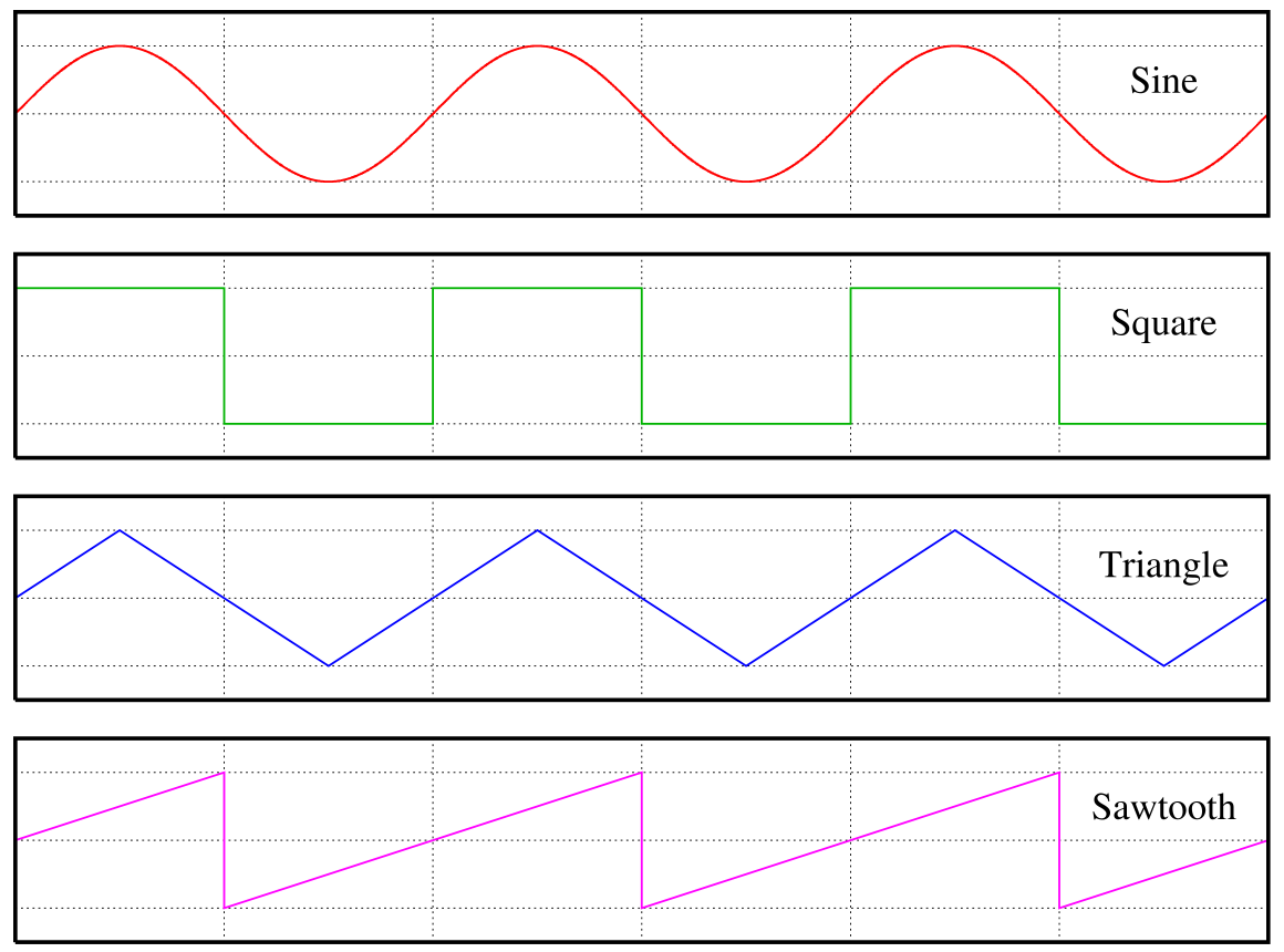
Sinusoids are a particular set of periodic signals; their defining characeristic is their relationship to angles and circles, e.g. sine and cosine
It’s important to remember that inputs to sinusoids (the independent variable) always has to be an angle (measured in radians). Therefore if we’re studying a sinusoidal signal as a function of time $t$ we need to be clear about what is the physical variable and what is the rescaled variable; consider that $\cos(2\pi t)$ has a period of $1$ second and a frequency of $1\text{Hz}$ (because it repeats when $t=0$ and $t=1$) but $\cos(t)$ has a period of $2\pi$ seconds and a frequency of $\frac{1}{2\pi} \text{Hz}$. For this reason (to clarify the ambiguity) sinusoids are usually written as $\cos(\omega t)$ where $\omega$ is called the angular frequency includes the conversion factor $2 \pi$ and and the frequency, i.e.
\[\omega = 2\pi f = \frac{2\pi}{T}\]Note that $\omega$ has units of radians per second, which fits as a unit for something that measures how many “angles” before a function repeats.
There are two more numbers that are essential for determining everything about a periodic signal: phase shift and amplitude. The phase shift $\phi$ of a periodic signal is how much of a “head start” the signal gets, e.g. for a sinusoid if the signal starts at its value at $\pi/4$ (90°) then the phase shift is $\phi = \pi/4$. Such a signal would be represented as $x(t) = \cos(\omega t + \phi) = \cos(\omega t + \pi/4)$. Notice that at $x(0) = \cos(\pi/4)$, hence “head start”. Notice also that $\phi = \pi/4$ and $\phi = 2\pi + \pi/4$ will produce the same “head start”, i.e.
\[x(0) = \cos(\phi) = \cos(2\pi + \pi/4) = \cos(\pi/4)\]because cosine is $2\pi$ periodic. This will be important later.
The final number that determines properties of the periodic functions is the amplitude $a$. It simply scales the values that the signal takes on, e.g. $5\cos(\omega t)$ takes on values in the range $[-5,5]$. Here’s an example for the signal $x(t) = 3\cos(100t - 0.01)$
Fourier series
Superposition
Suppose you have two periodic signals with the same periods, phases, and amplitudes
\[\begin{eqnarray*} x(t) = a \cos(\omega t + \phi) \\ y(t) = a \cos(\omega t + \phi) \end{eqnarray*}\]and you combined them additively, i.e. $s(t) = x(t) + y(t)$. What does the “resultant” signal look like? Well it’s simple: they’ll just reinforce each other
\[\begin{eqnarray*} s(t) &=& x(t) + y(t) \\ &=& a \cos(\omega t + \phi) + a \cos(\omega t + \phi) \\ &=& (a+a) \cos(\omega t + \phi) \\ &=& 2a \cos(\omega t + \phi) \end{eqnarray*}\]So the resulting signal will have the same period and phase as the constituent signals but will have twice the amplitude. This is called constructive interference. What about if $x(t)$ and $y(t)$ had exactly opposite amplitudes. Then the signals would cancel each other out
\[s(t) = (-a) \cos(\omega t + \phi) + a \cos(\omega t + \phi) = (-a+a) \cos(\omega t + \phi) = 0\]This is called destructive interference.
Now what about two signals that don’t have the same amplitudes, periods, and phases? Can you additively combine them as well? Sure, why not; the resultant signal doesn’t have a simple representation but if you think of signals as functions, which they are, combining distinct signals in this way is the same as adding functions (which itself simply means adding the values that the functions “output” for a particular value of the input). You can then generalize this kind of additive combination to any number of signals. In general this is called superposition.
Decomposition
Okay so you can combine periodic signals easily enough. Can you also reverse the process? Can you decompose signals into their constituent parts (i.e. periodic signals)? It turns out that in fact you can. To motivate the process let’s for the moment take the case where you know your aggregate (combined) signal $s(t)$ consists of two sinusoidal signals $x(t) = \cos(2 \pi f_x t) $ and $y(t) = \cos(2 \pi f_y t)$ and you know the frequencies $f_x, f_y$ but you don’t know how much each frequency contributes, i.e.
\[s(t) = a_x x(t) + a_y y(t) = a_x \cos(2 \pi f_x t) + a_y \cos(2 \pi f_y t)\]and you need to determine $a_x, a_y$. In a sense you need to “isolate” the contribution of each component frequency.
If you think a little abstractly this might remind you of finding the components of a vector relative to the standard basis
\[\vec{z} = \vec{x} + \vec{y} = a_x \vec{e_1} + a_y \vec{e_2} = a_x\begin{bmatrix}1\\ 0\end{bmatrix} + a_y\begin{bmatrix}0\\ 1\end{bmatrix}\]In this case you “isolate” the contribution of each component using a “trick” involving the dot product:
\[\vec{z} \cdot \vec{e_1} = a_x \vec{e_1} \cdot \vec{e_1} + a_y\cancelto{0}{\vec{e_2} \cdot \vec{e_1}} = a_x \cdot 1\]and so $a_x = \vec{z} \cdot \vec{e_1}$. Geometrically this is called the projection of $\vec{z}$ onto $e_1$ and the “trick” works because the dot product is actually an inner product. The details of the theory aren’t super important; the point is simply that you can think of decomposing periodic signal into component frequencies just like you think of decomposing a vector into coordinate axes components. Indeed the trick we use to isolate the frequency components uses a suitably defined inner product for signals/functions: the integral
\[\int_{0}^{1} s(t) \cos(2 \pi f_x t) dt = \int_{0}^{1}a_x \cos(2 \pi f_x t) \cos(2 \pi f_x t) dt + \int_{0}^{1} a_y \cos(2 \pi f_y t) \cos(2 \pi f_x t) dt\]This integral against $\cos(2 \pi f_x t)$ on both sides is the trick itself. Let’s perform each of the integrals on the right carefully; let’s start with the second using angle sum and product identities
\[\int_{0}^{1}a_y \cos(2 \pi f_y t) \cos(2 \pi f_x t) dt = \frac{a_y}{2} \int_{0}^{1} \cos(2 \pi (f_y - f_x) t) + \cos(2 \pi (f_y + f_x) t) dt\]Since $f_y \neq f_x$ each of the cosines on the right hand side are just integrals of $\cos$ over multiple periods, which is zero because $\cos$ symmetric around the $y$-axis

So $\int_{0}^{1}a_y \cos(2 \pi f_y t) \cos(2 \pi f_x t) dt = 0$ but
\[\begin{eqnarray*} \int_{0}^{1}a_x \cos(2 \pi f_x t) \cos(2 \pi f_x t) dt &=& \frac{a_x}{2} \int_{0}^{1} \cos(2 \pi (f_x - f_x) t) + \cos(2 \pi (f_x + f_x) t) dt \\ &=& \frac{a_x}{2} \int_{0}^{1} \cos(2 \pi \cdot 0 \cdot t) + \cos(2 \pi (2f_x) t) dt \\ &=& \frac{a_x}{2} \int_{0}^{1} 1dt + \frac{a_x}{2} \cancelto{0}{ \int_{0}^{1}\cos(2 \pi (2f_x) t) dt }\\ &=& \frac{a_x}{2} \end{eqnarray*}\]and hence finally to figure out $a_x$ we have that
\[\int_{0}^{1} s(t) \cos(2 \pi f_x t) dt = \frac{a_x}{2} \iff a_x = 2 \int_{0}^{1} s(t) \cos(2 \pi f_x t) dt\]Similarly
\[a_y = 2 \int_{0}^{1} s(t) \cos(2 \pi f_y t) dt\]It’s important you soke all of that in because it is the basis for all of signal processing!
I encourage you to look at these two expressions and understand the first in terms of the second
\[a_x = 2 \int_{0}^{1} s(t) \cdot \cos(2 \pi f_x t) dt \iff a_x = \vec{z} \cdot \vec{e_1}\]The periodic functions $\cos(2\pi f t)$ and $\sin(2 \pi f t)$ play the role of the basis vectors $\vec{e_1}, \vec{e_2}, \dots$ and just like how for basis vectors it’s true that
\[\vec{e_i} \cdot \vec{e_j} = \begin{cases} 1 & i = j \\ 0 & i \neq j \\ \end{cases}\]it’s also true for sines and cosines
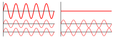
\[\begin{eqnarray*} \int_{0}^{1} \cos(2 \pi f_x t) \cdot \cos(2 \pi f_y t) dt &=& \begin{cases} 1 & f_x = f_y \\ 0 & f_x \neq f_y \\ \end{cases} \\ \\ \int_{0}^{1} \sin(2 \pi f_x t) \cdot \sin(2 \pi f_y t) dt &=& \begin{cases} 1 & f_x = f_y \\ 0 & f_x \neq f_y \\ \end{cases} \\ \\ \int_{0}^{1} \cos(2 \pi f_x t) \cdot \sin(2 \pi f_y t) dt &=& 0 \end{eqnarray*}\]Here’s geometric “proof” of all off the above identities

Definition
Let’s recap: you can combine periodic signals to produce new periodic signals. You can also decompose simple (sinusoids) periodic signals into their components, each of those components itself being a periodic signal (sinusoid) with a particular frequency. Drum roll please: it is true that absolutely any period signal (not just sinusoids) can be decomposed into sum of sines and cosines. This is akin to magic and the only caveat is that the sum might be infinite. The precise formula for the Fourier series expansion of a periodic function $s(t)$ is
\[s(t) = {\frac {1}{2}}a_{0}+\sum _{n=1}^{\infty }[a_{n}\cos(2\pi \ n\ t)+b_{n}\sin(2\pi \ n\ t)]\]where $f = n$, i.e. integer frequencies, and $a_0$ is related to the average of $s(t)$ and serves the role shifting the expansion up and down
\[a_0 = 2\int_0^1 s(t) dt\]The coefficients $a_i, b_i$ are computed just like how we computed them in the two component case
\[a_{n}=2\int _{0}^{1}s(t)\cos(2\pi \ n\ t)\;dt\quad {\text{and}}\quad b_{n}=2\int _{0}^{1}s(t)\sin(2\pi \ n\ t)\;dt\]The full formula includes sines for maximum generality (usefulness). For example some periodic signals are 0 at $t=0$ and can’t be represented using cosines (since $\cos(0)=1$).
The way you should think about Fourier series expansion formula is that you can represent any periodic function as a (possibly infinite) combination “simple” parts, i.e. just sines and cosines of different frequencies. How much each simple part (i.e. each frequency $n$) contributes is determined/controlled by the coefficients $a_n, b_n$.
Note that if you can’t use the infinite expansion (i.e. in practice) this is still very useful because it means you can very closely approximate any periodic function. For example the sawtooth function defined by
\[s(t)=t-\underbrace {\lfloor t\rfloor } _{\operatorname {floor} (t)}\]which looks like

has the expansion
\[\begin{aligned}s(t)&={\frac {a_{0}}{2}}+\sum _{n=1}^{\infty }\left[a_{n}\cos \left(nt\right)+b_{n}\sin \left(nt\right)\right]\\left[4pt]&={\frac {2}{\pi }}\sum _{n=1}^{\infty }{\frac {(-1)^{n+1}}{n}}\sin(nt)\end{aligned}\]and you can see that a progressive sum of the first five terms of the series
already fairly closely approximates it, i.e.
\[s(t) \sim {\frac {2}{\pi }} \left( \frac{\sin(1t)}{1} + \frac{-\sin(2t)}{2} + \frac{\sin(3t)}{3} + \frac{-\sin(4t)}{4} + \frac{\sin(5t)}{5} \right)\]is already very close to the sawtooth function.
Frequency space
Notice that the Fourier series expansion gives an equivalent way of specifying any periodic function $s(t)$; you can either give the values $s(t)$ takes on over time, called time domain representation (this is the conventional way you’re used to) or you can give the frequencies $f_n$ and the coefficients $a_n, b_n$ of the fourier series expansion, called frequency domain representation. For example the inverse sawtooth wave can be specified as
\[s(t)=A - \frac {At}{T}\quad {\text{for }}kT\leq t<(k+1)T\]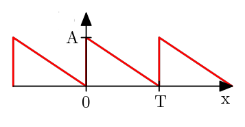
can be represented in frequency domain as
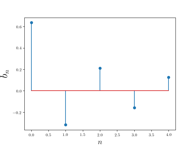
\[\begin{eqnarray*} a_{0}&=&A\\ a_{n}&=&0\\ b_{n}&=&\frac {A}{n\pi }\\ \end{eqnarray*}\]Here is a plot of the frequencies and their corresponding weights
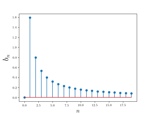
Let’s take a minute to reflect on how this representation differs from the time domain representation (the conventional one). First, notice that the plot of component coefficients $b_n$ versus frequencies $n$ is not continuous. This is because we only consider sines and cosines with integer $n$ frequencies ($n =1,2,3,4, \dots$). Second, and more important, notice that the contribution of each frequency (as measured by $b_n$) drops off very quickly after the first 3 or 4 components ($b_4$ is already $1/4$ of $b_1$). If you look at the time domain plot of the sawtooth this should make sense; the sawtooth function doesn’t change very quickly over small spans of time (which is exactly the effect of a high frequency component in a periodic signal). This kind of analysis of a signal is difficult in time domain but very easy in the frequency domain.
Filters
If analysis were the only thing frequency domain representation (and therefore Fourier series) were useful for it would already be worth the time investment to learn but in fact it’s the transformations on the signal that you can perform in frequency domain that make it truly useful. Let’s take the our five term expansion of the sawtooth
\[s(t) \sim {\frac {2}{\pi }} \left( \frac{\sin(1t)}{1} + \frac{-\sin(2t)}{2} + \frac{\sin(3t)}{3} + \frac{-\sin(4t)}{4} + \frac{\sin(5t)}{5} \right)\]It has a frequency domain representation
It looks like
Now let’s “filter” the highest two frequencies (which amounts to setting their coefficients to 0)
\[s(t) \sim {\frac {2}{\pi }} \left( \frac{\sin(1t)}{1} + \frac{-\sin(2t)}{2} + \frac{\sin(3t)}{3}\right)\]which has the frequency domain representation
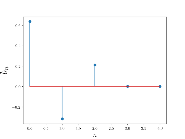
It now looks like
It might not be immediately obvious but the result is that the function is now smoother; with fewer high frequency components the function changes values much more slowly.
If you think of the frequency domain representation as a vector
\[s[n] = \left[\frac{2}{\pi},\frac{-4}{\pi},\frac{6}{\pi},\frac{-8}{\pi},\frac{10}{\pi}\right]\]and the transformed frequency domain representation also as a vector
\[H[n] = \left[\frac{2}{\pi},\frac{-4}{\pi},\frac{6}{\pi},0,0\right]\]then this filter can thought of as a dot product with the vector $\left[1,1,1,0,0\right]$
\[s[n]\cdot H[n] = \left[\frac{2}{\pi},\frac{-4}{\pi},\frac{6}{\pi},\frac{-8}{\pi},\frac{10}{\pi}\right] \cdot \left[1,1,1,0,0\right] = \left[\frac{2}{\pi},\frac{-4}{\pi},\frac{6}{\pi},0,0\right]\]which is equivalent to multiplying a “box” function
\[H[n] = \begin{cases} 1 & n \in {1,2,3} \\ 0 & \text{otherwise} \\ \end{cases}\]with the frequency domain representation
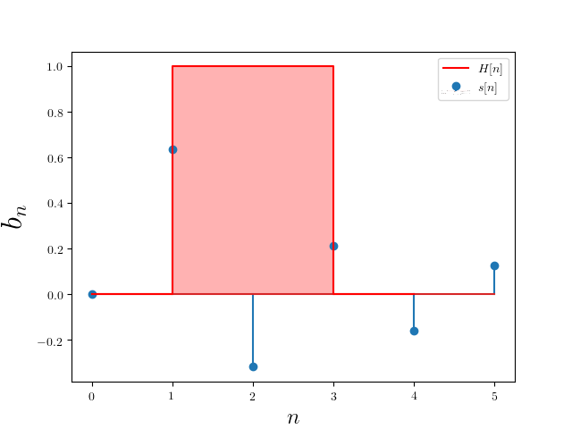
and multiply the box function and the frequency domain representation. Since the box function is constant 1 over the relevant frequencies and zero otherwise it produces the same filtering effect.
This is called applying a low pass filter because it lets only low frequencies pass through (the filter).
Just in case you’re interested this kind of thing can actually be implemented using electrical components.
Interlude: complex numbers
The real numbers $\mathbb{R}$ are typical numbers we all know and love, numbers like $0,1,2,\pi,\sqrt{2}, -1, 42$ etc. Unfortunately if they’re the only numbers we can choose from we can’t solve equations like $x^2 = -1$. Quite unfortunate. So what do we do as sophisticated mathematicians? Simply define $i$ to be the solution of $x^2 = -1$, i.e. $i = \sqrt{-1}$ and throw it in the with the rest of the real numbers. The result if is a set of numbers where each number has two “parts”: a real part, a conventional real quantity, and a complex part, a quantity that is scalar multiple of $i$. One way to represent complex numbers is as a pair $(a, bi)$ where $a$ is the real part and $bi$ is the complex part, the scalar multiple of $i$. Addition of complex numbers is defined entry-wise:
\[(a, bi) + (c, di) = (a+c, (b+d)i)\]Multiplication is more complicated
\[(a, bi) \times (c, di) = (ac-bd, (ad+cb)i)\]There’s another way to represent complex numbers that makes these rules (at least multiplication) more natural: $a+bi$. Then both addition and multiplication proceeds just like it does for polynomials (addition between terms with the same $i$ coefficient and multiplication according to “FOIL”).
\[(a+bi) + (c+di) = (a+b)+(c+d)i\]and
\[(a+bi)\times(c+di) = ac + adi + cbi + bdi^2 = (ac - bd) + (ad+cb)i\]where I used the fact that $i = \sqrt{-1} \implies i^2 = -1$.
Given that complex numbers can be thought as consisting of two parts they can be plotted on a two axis plot
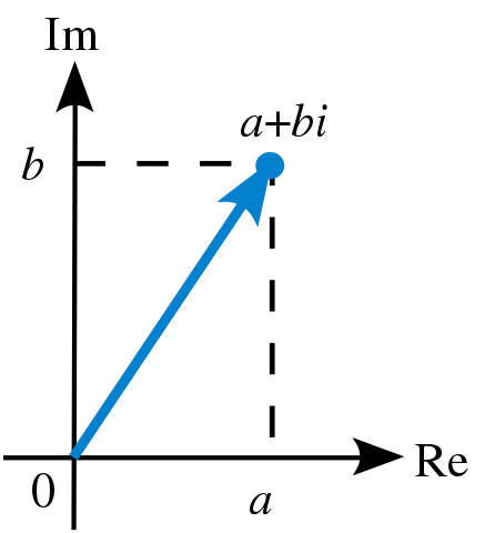
and therefore an equivalent representation in terms of angles
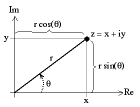
This is called an Argand diagram and the representation is called the polar representation of a complex number. In particular $z = r (\cos(\theta) + i \sin(\theta))$. Using this representation there’s another useful form of a complex number we can construct; using euler’s identity
\[z = r e^{i \theta} = r (cos(\theta) + i \sin(\theta))\]Using this exponential/polar form of complex numbers we can write down a much more compact Fourier series representation of a periodic signal. Starting with expressing $\cos(\theta)$ and $\sin(\theta)$ in terms of the complex exponential
\[\begin{eqnarray*} e^{i\theta} + e^{i(-\theta)} &=& (cos(\theta) + i \sin(\theta)) + (cos(-\theta) + i \sin(-\theta)) \\ &=& (cos(\theta) + i \sin(\theta)) + (cos(\theta) - i \sin(\theta)) \\ &=& 2\cos(\theta) \end{eqnarray*}\]since cosine is an even function and sine is an odd function. Similarly
\[e^{i\theta} - e^{i(-\theta)} = 2i\sin(\theta)\]Therefore
\[\begin{eqnarray*} \cos(\theta) &=& \frac{1}{2}\left(e^{i\theta} + e^{i(-\theta)}\right) \\ \sin(\theta) &=& \frac{1}{2i}\left(e^{i\theta} - e^{i(-\theta)}\right) \end{eqnarray*}\]and hence
\[\begin{eqnarray*} s(t) &=& {\frac {1}{2}}a_{0}+\sum _{n=1}^{\infty }[a_{n}\cos(2\pi \ n\ t)+b_{n}\sin(2\pi \ n\ t)] \\ &=& {\frac {1}{2}}a_{0}+\sum _{n=1}^{\infty }\left[\frac{a_n}{2}\left(e^{i 2 \pi n t} + e^{-i2 \pi n t}\right)+\frac{b_n}{2i}\left(e^{i 2 \pi n t} - e^{-i2 \pi n t}\right) \right] \\ &=& {\frac {1}{2}}a_{0}+\sum _{n=1}^{\infty }\left[\frac{1}{2}\left(a_n + ib_n\right)e^{i2\pi n t}\right] \\ && +\sum _{n=1}^{\infty }\left[\frac{1}{2}\left(a_n - ib_n\right)e^{-i2\pi n t}\right] \\ &=& \sum _{n=-\infty}^{\infty }u_ne^{i2\pi n t}\\ \end{eqnarray*}\]where
\[u_n = \begin{cases} \frac{1}{2}\left(a_n + ib_n\right) &{\text{if }}n\geq1\\ \frac{a_0}{2} &{\text{if }}n=0\\ \frac{1}{2}\left(a_n - ib_n\right) &{\text{if }} n \leq -1 \end{cases}\]But actually you can calculate $u_n$ from first principles, in a similar fashion to how we originally calculated $a_n, b_n$
\[\begin{eqnarray*} \int_0^1 s(t)e^{-i2\pi m t} dt &=& \int_0^1 \sum _{n=-\infty}^{\infty }u_ne^{i2\pi n t}e^{-i2\pi m t} dt\\ &=& \sum _{n=-\infty}^{\infty }u_n\int_0^1 e^{i2\pi (n-m) t} dt\\ &=&\begin{cases} u_n (1+0i) &{\text{if }}n = m\\ u_n (0+0i) &{\text{if }} n \neq m \end{cases} \end{eqnarray*}\]by the same integrals we performed in decomposition.
Hence the exponential form of the Fourier series is
\[\begin{eqnarray*} s(t) &=& \sum _{n=-\infty}^{\infty }u_ne^{i2\pi n t}\\ u_n &=& \int_0^1 s(t)e^{-i2\pi n t} dt \end{eqnarray*}\]From now on we’ll use this form because all of the algebra and calculus is easier.
Notice that in this representation the frequencies $n$ range over negative values as well as positive values. For example notice that
\[\begin{eqnarray*} \cos(2\pi t) &=& \frac{1}{2}e^{i2\pi \cdot (1) t} + \frac{1}{2} e^{i 2\pi \cdot (-1) t} \\ \end{eqnarray*}\]has frequency components $1$ and $-1$ with equal weights $\frac{1}{2}$. This is true in general: a physical signal has a frequency spectrum that is symmetric around 0.
Fourier transform
The Fourier series is useful for studying the frequency space representation of a periodic, continuous time signal. We’ll eventually get to studying discrete time signals but for right now let’s consider continuous time aperiodic signals. For example the unit pulse function
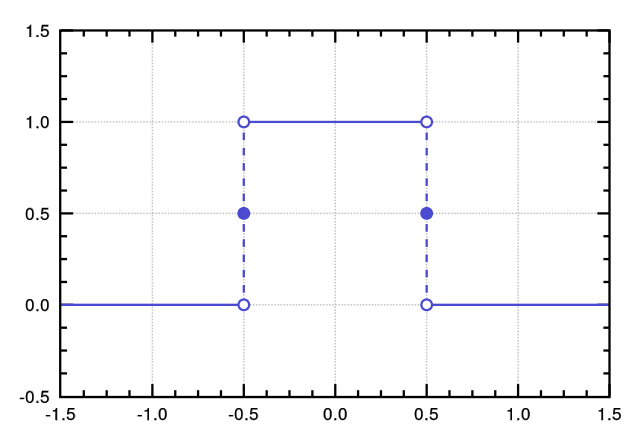
defined by
\[\operatorname {rect} (t)=\Pi (t)= \begin{cases} 0,&{\text{if }}|t|>{\frac {1}{2}}\\ {\frac {1}{2}},&{\text{if }}|t|={\frac {1}{2}}\\ 1,&{\text{if }}|t|<{\frac {1}{2}} \end{cases}\]This function, because it’s not periodic, cannot be represented as a fourier series. What we can do is represent the “periodic continuation” of the unit pulse
defined by
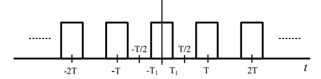
\[\pi (t)= \begin{cases} 0,&{\text{if }}T_1 < |t|<{\frac {T}{2}} \\ 1,&{\text{if }}|t|< T_1 \end{cases}\]Square wave
The square wave is a periodic signal with period $T$ and frequency $\omega_0 = 2\pi/T$ and $T_1$ is half the width (in time). What are the fourier series coefficients for this signal? Before we can calculate them we need to adjust the formula for the coefficients because $\pi(t)$ is $\left[0, T\right]$ periodic rather than $\left[0, 1\right]$ periodic (like $\cos(2 \pi t)$ and $\sin(2\pi t)$ in our original definition). In order for the basis functions (either the complex exponentials or sines/cosines) to have the same periodicity as $\pi(t)$ we need to scale $t$ by $1/T$, i.e. $e^{- i (2 \pi/T) t}$ is periodic in $T$ (plug in some values of $t$ to see for yourself). Therefore let’s introduce the change of variable $\tau/T = t$. Then $t = 0 \implies \tau = 0$ and $t = 1 \implies \tau = T$ and $dt = (1/T)d\tau$. This transforms the integral for $u_n$ into
\[u_n =\frac{1}{T} \int_0^T \pi(\tau)e^{-i \frac{2\pi}{T} n \tau} d\tau\]at which point it makes sense to use the fundamental frequency $\omega_0 = 2\pi/T$
\[u_n =\frac{1}{T} \int_0^T \pi(\tau)e^{-i \omega_0 n \tau} d\tau\]and since the variable of integration doesn’t actually matter we return to using $t$ instead of $\tau$
\[u_n =\frac{1}{T} \int_0^T \pi(t)e^{-i \omega_0 n t} dt\]This formula is correct but it’s actually more convenient to integrate over $\left[-T/2, T/2\right]$ since $\pi(t)$ is symmetric on that interveral. Also note that $\pi(t)$ is zero for $T_1 < |t|<{\frac {T}{2}}$ so we actually only need to integrate over $\left[-T_1, T_1\right]$. Hence the final integration for the coefficients is
\[u_n =\frac{1}{T} \int_{-T_1}^{T_1} \pi(t)e^{-i \omega_0 n t} dt = \frac{1}{T} \int_{-T_1}^{T_1} 1\cdot e^{-i \omega_0 n t} dt\]Hence
\[u_0 = \frac{1}{T} \int_{-T_1}^{T_1} 1\cdot e^{-i \omega_0 \cdot0 \cdot t} dt = \frac{2T_1}{T}\]and for $k \neq 0$
\[\begin{eqnarray*} u_k &=& \frac{1}{T} \int_{-T_1}^{T_1} 1\cdot e^{-i \omega_0 \cdot k \cdot t} dt \\ &=& -\frac{1}{ik\omega_0 T} e^{- i k \omega_0 t} \Bigg|_{-T_1}^{T_1} \\ &=& \frac{2}{k\omega_0 T} \left( \frac{e^{i k \omega_0 T}- e^{-i k \omega_0 T}}{2i} \right) \\ &=& \frac{2 \sin(k \omega_0 T)}{k \omega_0 T} \end{eqnarray*}\]The first 30 coefficients ($-30$ to $30$) looks like
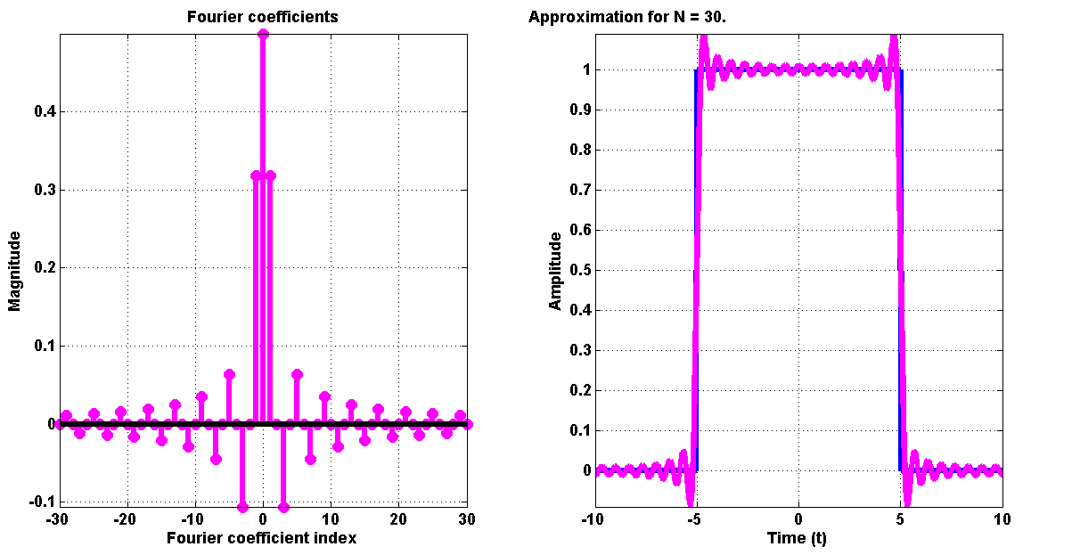
Notice that the spectrum is symmetric - this was mentioned towards the end of the complex numbers section.
Unit pulse as a limit
Back to the unit pulse function.
Let’s actually look at the square wave spectrum rescaled by $T$, i.e.
\[T u_k = \frac{2 \sin (k \omega_0 T_1)}{k \omega_0}\]If you think of $\omega = \omega_0 k$ as a continuous parameter then this becomes
\[\frac{2 \sin (\omega T_1)}{\omega}\]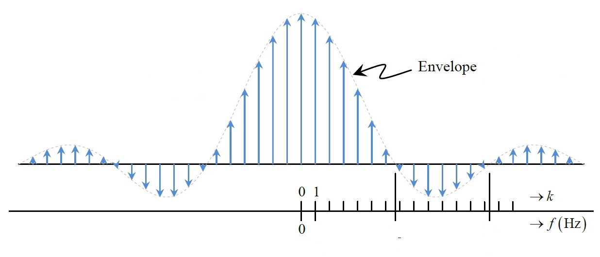
which can be thought of as the “envelope” for the scaled coefficients $T u_k$, i.e. to get $T u_k$ sample the function $2 \sin (\omega T_1)/\omega$ at values $ \omega = \omega_0 k$. Also notice that as $T$ increases (and $\omega_0$ decreases since $\omega_0 = 2 \pi /T$ ) the samples will have to be spaced closer and closer together. Simultaneously, as $T$ increases, the spacing between individual “lobes” of the square wave move farther and farther apart, until in the limit we have just one lobe of the rectangular pulse.
“Derivation”
The argument as applied to the rectangular pulse bears out for arbitrary aperiodic signal; let $x(t)$ be such a signal that’s zero outside of some interval $T$, for simplicity’s sake symmetric around $t=0$. Then since outside of the $T$ interval $x(t) = 0$ it’s the case that
\[\begin{eqnarray*} u_k &=& \frac{1}{T} \int_{-T/2}^{T/2} x(t) \cdot e^{-i \omega_0 t} dt \\ &=& \frac{1}{T} \int_{-\infty}^{\infty} x(t) \cdot e^{-i \omega_0 t} dt \\ \end{eqnarray*}\]Defining $X(\omega)$ as the envelope of the scaled coefficients $T u_k$
\[X(\omega) = \int_{-\infty}^{\infty} x(t) \cdot e^{-i \omega t} dt\]we have that
\[u_k = \frac{1}{T} X(k \omega_0)\]and then the fourier series representation becomes
\[x(t) =\frac{1}{T} \sum_{k=-\infty}^{\infty} X(k \omega_0)e^{i k \omega_0 t}\]or equivalently, since $2 \pi/T = \omega_0$
\[x(t) =\frac{1}{2\pi} \sum_{k=-\infty}^{\infty} X(k \omega_0)e^{i k \omega_0 t} \omega_0\]Taking $T \rightarrow \infty$ or equivalently $\omega_0 \rightarrow 0$ such that $\omega = \omega_0 k$ stays constant, the sum becomes an integral and
\[x(t) =\frac{1}{2\pi} \int_{-\infty}^{\infty} X(\omega)e^{i \omega t} d\omega\]Therefore the Fourier transform is defined by
\[\begin{eqnarray*} X(\omega) &=& \int_{-\infty}^{\infty} x(t) \cdot e^{-i \omega t} dt \\ x(t) &=& \frac{1}{2\pi} \int_{-\infty}^{\infty} X(\omega)e^{i \omega t} d\omega \end{eqnarray*}\]