
Tensor Networks for Simulating Quantum Circuits on FPGAs
Most research in quantum computing today is performed against simulations of quantum computers rather than true quantum computers. Simulating a quantum computer entails implementing all of the unitary operators corresponding to the quantum gates as tensors. For high numbers of qubits, performing tensor multiplications for these simulations becomes quite expensive, since $N$-qubit gates correspond to $2^{N}$-dimensional tensors. One way to accelerate such a simulation is to use field programmable gate array (FPGA) hardware to efficiently compute the matrix multiplications. Though FPGAs can efficiently perform tensor multiplications, they are memory bound, having relatively small static random access memory. One way to potentially reduce the memory footprint of a quantum computing system is to represent it as a tensor network; tensor networks are a formalism for representing compositions of tensors wherein economical tensor contractions are readily identified. Thus we explore tensor networks as a means to reducing the memory footprint of quantum computing systems and broadly accelerating simulations of such systems.
Introduction
Quantum computing (QC) refers to the manipulation and exploitation of properties of quantum mechanical (QM) systems to perform computation. QM systems exhibit properties such as superposition and entanglement and clever quantum algorithms operate on these systems to perform general computation. Unsurprisingly, the technique was initially conceived of as a way to simulate physical systems themselves:
“… [N]ature isn’t classical, dammit, and if you want to make a simulation of nature, you’d better make it quantum mechanical, and by golly it’s a wonderful problem, because it doesn’t look so easy.”
This closing remark from the keynote at the 1st Physics of Computation Conference in 1981, delivered by the late Richard Feynman [1], succinctly, but accurately, expresses that initial goal of quantum computing. Although modeling and simulating physical systems on quantum computers remains a thriving area of research we narrow our focus here to QC as it pertains to solving general computational problems. Such problems include unstructured search [2], integer factorization [3], combinatorial optimization [4], and many others. It is conjectured that some quantum algorithms enable quantum computers to exceed the computational power of classical computers [5].
QC systems are composed of so-called quantum bits, or qubits, that encode initial and intermediate states of computations. Transformations between states are effected by time-reversible transforms, called unitary operators. A formalism for representing quantum computation is the quantum circuit formalism, where semantically related collections of $N$ qubits are represented as registers and transformations are represented as gates, connected to those registers by wires, and applied in sequence. As already mentioned, in hardware, quantum circuits correspond to physical systems that readily exhibit quantum technical properties; examples of physical qubits include transmons, ion traps and topological quantum computers [6]. Current state of the art QC systems are termed Noisy Intermediate-Scale Quantum (NISQ) systems. Such systems are characterized by moderate quantities of physical qubits (50-100) but relatively few logical qubits (i.e. qubits robust to interference and noise). Due to these limitations (and, more broadly, the relative scarcity of functioning QC systems), most research on quantum algorithms is performed with the assistance of simulators of QC systems. Such simulators perform simulations by representing $N$-qubit circuits as $2^{N}$-dimensional complex vectors and transformations on those vectors as $2^{N}$-dimensional complex matrix-vector multiplication. Naturally, due to this exponential growth, naively executing such simulations quickly become infeasible for $N>50$ qubits [7], both due to memory constraints and compute time.
It’s the case that matrices are a subclass of a more general mathematical object called a tensor and composition of matrices can be expressed as tensor contraction. Tensor networks (TNs) are decompositions (i.e. factorizations) of very high-dimensional tensors into networks (i.e. graphs) of low-dimensional tensors. TNs have been successfully employed in reducing the memory requirements of simulations of QC systems [7]. The critical feature of tensor networks that make them useful for QC is the potential to perform tensor contractions on the low-dimensional tensors in an order such that, ultimately, the memory and compute time requirements are lower than for the traditional representation. Existing applications of TNs to quantum circuits focus primarily on memory constraints on general purpose computers [8] and distributed environments [9].
FPGAs are known to be performant for matrix multiplication uses cases [10]. Though FPGAs typically run at lower clock speeds (100-300MHz) than either conventional processors or even graphics processors they, nonetheless, excel at latency constrained computations owing to their fully “synchronous” nature (all modules in the same clock domain execute simultaneously). At first glance FPGAs seem like a suitable platform for performant simulation of quantum systems when runtime is of the essence. Unfortunately, RAM is one of the more limited resources on an FPGA and therefore it becomes necessary to explore memory reduction strategies for simulations (as well as runtime reduction strategies). Hence, we explore tensor networks as a means of reducing the memory footprint of quantum circuits with particular attention to dimensions of the designs space as they pertain to deployment to FPGAs.
The remainder of this report is organized as follows: section Background covers the necessary background wherein subsection Quantum-Computing very briefly reviews quantum computation and quantum circuits (with particular focus on aspects that will be relevant for tensor networks and FPGAs), section Tensors-and-Tensor-Networks defines tensors and tensor networks fairly rigorously and discusses algorithms for identifying optimal contraction orders, section FPGAs discusses the constraints imposed by virtue of deploying to FPGA, section Implementation describes our implementation of TNs on FPGAs, section Evaluation reports our results on various random circuits, and section Conclusion concludes with future research directions.
Background
Quantum Computing
We very (very) quickly review quantum computing and quantum circuits as they pertain to our project. For a much more pedagogically sound introduction consult [11]. As already alluded to, quantum computing exploits properties of quantum mechanical systems in order to perform arbitrary computation. The fundamental unit of quantum computation is a qubit, defined as two-dimensional quantum system with state vector $\psi$ an element of a Hilbert space1 $H$:
\[\psi:=\alpha\begin{pmatrix}1\\ 0 \end{pmatrix}+\beta\begin{pmatrix}0\\ 1 \end{pmatrix}\equiv\begin{pmatrix}\alpha\\ \beta \end{pmatrix}\]where $\alpha,\beta\in\mathbb{\mathbb{C}}$ and $\left|\alpha\right|^{2}+\left|\beta\right|^{2}=1$. This exhibits the superposition property of the qubit2 in that the squares of the coefficients are the probabilities of measuring the system in the corresponding basis state. Collections of qubits have state vectors that represented by the tensor product of the individual states of each qubit; for example, two qubits $\psi,\phi$ have state vector
\[\psi\otimes\phi:=\begin{pmatrix}\alpha\\ \beta \end{pmatrix}\otimes\begin{pmatrix}\alpha'\\ \beta' \end{pmatrix}\equiv\begin{pmatrix}\alpha\alpha'\\ \alpha\beta'\\ \beta\alpha'\\ \beta\beta' \end{pmatrix}\]where the second $\otimes$ is the Kronecker product and $\alpha\alpha’$ indicates conventional complex multiplication. Note that the basis relative to which $\psi\otimes\phi$ is represented is the standard basis for $\mathbb{C}^{4}$ and thus we observe exponential growth in the size of the representation of an $N$-qubit system. An alternative notation for state vectors is Dirac notation; for example, for a single qubit
\[\ket{\psi}\equiv\alpha\ket{0}+\beta\ket{1}\]and a 2-qubit system
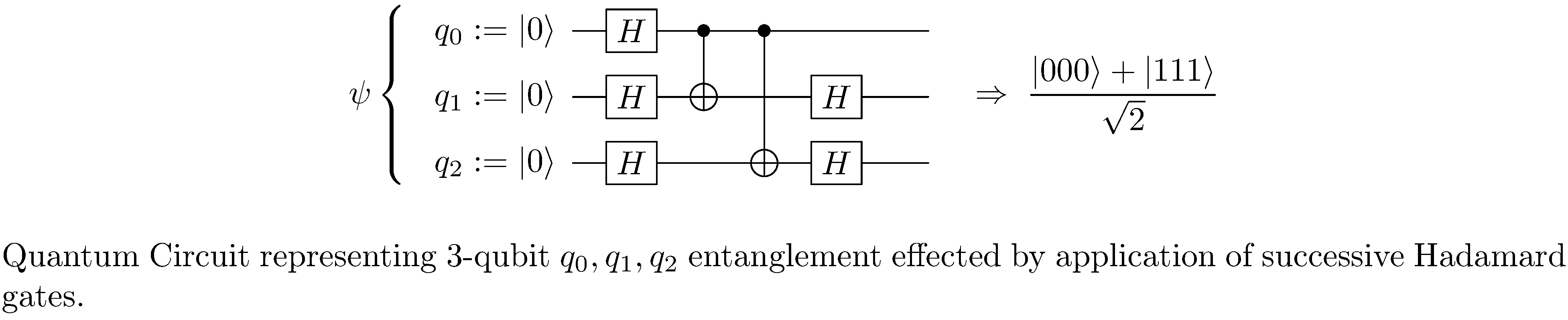
\[\begin{aligned} \ket{\psi}\otimes\ket{\phi} & \equiv\left(\alpha\ket{0}+\beta\ket{1}\right)\otimes\left(\alpha'\ket{0}+\beta'\ket{1}\right)\\ & \equiv\alpha\alpha'\ket{0}\otimes\ket{0}+\alpha\beta'\ket{0}\otimes\ket{1}+\beta\alpha'\ket{1}\otimes\ket{0}+\beta\beta'\ket{1}\otimes\ket{1}\\ & \equiv\alpha\alpha'\ket{0}\ket{0}+\alpha\beta'\ket{0}\ket{1}+\beta\alpha'\ket{1}\ket{0}+\beta\beta'\ket{1}\ket{1}\\ & \equiv\alpha\alpha'\ket{00}+\alpha\beta'\ket{01}+\beta\alpha'\ket{10}+\beta\beta'\ket{11}\\ & \equiv\alpha\alpha'\ket{0}+\alpha\beta'\ket{1}+\beta\alpha'\ket{2}+\beta\beta'\ket{3}\end{aligned}\]where in the last line we’ve used the decimal representation for the bit strings identifying the basis states. Of particular import for QC are the entangled or bell states; they correspond to multi-qubit states, such as
\[\ket{\xi}=\frac{1}{\sqrt{2}}\ket{00}+\frac{1}{\sqrt{2}}\ket{11}\]that cannot be “factored” into component states3. Then, naturally, changes in qubit states are represented as unitary4 matrices $U$; for example
\[\psi'=U\psi=\begin{pmatrix}U_{00} & U_{01}\\ U_{10} & U_{11} \end{pmatrix}\begin{pmatrix}\alpha\\ \beta \end{pmatrix}=\begin{pmatrix}U_{00}\alpha+U_{01}\beta\\ U_{10}\alpha+U_{11}\beta \end{pmatrix}\]Matrix representations of transformations on multi-qubit states are constructed using the Kronecker product on the individual matrix representations; for example
\[U\otimes V:=\begin{pmatrix}U_{00}V & U_{01}V\\ U_{10}V & U_{11}V \end{pmatrix}:=\begin{pmatrix}U_{00}V_{00} & U_{00}V_{01} & U_{01}V_{00} & U_{01}V_{01}\\ U_{00}V_{10} & U_{00}V_{11} & U_{01}V_{10} & U_{01}V_{11}\\ U_{10}V_{00} & U_{10}V_{01} & U_{11}V_{00} & U_{11}V_{01}\\ U_{10}V_{10} & U_{10}V_{11} & U_{11}V_{10} & U_{11}V_{11} \end{pmatrix}\]Here we see again an exponential growth in representation size as a function of the number of qubits.
As already alluded to, quantum circuits are a formalism for representing quantum computation in general and algorithms designed for quantum computers in particular. In the quantum circuit formalism qubit states are represented by wires and unitary transformations are represented by gates (see figure 1), much like classical combinational logic circuits might be, though, whereas combinational logic is “memoryless”5, sequences of quantum gates specified by a quantum circuit do in fact connote the evolution (in time) of the qubits. In addition quantum gates, as opposed to classical gates, are necessarily reversible and hence there are no quantum analogs to some classical gates such as NOT and OR.
Tensors and Tensor Networks
We quickly define tensors and tensor networks and then move on to tensor network methods for simulating quantum circuits.
Tensors
One definition of a tensor6 $T$ is as an element of a tensor product space7:
\[T\in\underbrace{V\otimes\cdots\otimes V}_{p{\text{ copies}}}\otimes\underbrace{V^{*}\otimes\cdots\otimes V^{*}}_{q{\text{ copies}}}\]where $V^{*}$ is dual8 to $V$. Then $T$, in effect, acts a multilinear map
\[{\displaystyle T:\underbrace{V^{*}\times\dots\times V^{*}}_{p{\text{ copies}}}\times\underbrace{V\times\dots\times V}_{q{\text{ copies}}}\rightarrow\mathbb{R}}\]by “applying” $p$ elements from $V$ to $p$ elements of $V^{*}$ and $q$ elements from $V^{*}$ to $q$ elements of $V$. Note the swapping of the orders of $V,V^{*}$ in both the definitions and the description. $T$’s coordinate basis representation
\[{\displaystyle T\equiv T_{j_{1}\dots j_{q}}^{i_{1}\dots i_{p}}\;\mathbf{e}_{i_{1}}\otimes\cdots\otimes\mathbf{e}_{i_{p}}\otimes\mathbf{e}^{j_{1}}\otimes\cdots\otimes\mathbf{e}^{j_{q}}}\label{eq:tensor_coord}\]is determined by its evaluation on each set of bases
\[{\displaystyle T_{j_{1}\dots j_{q}}^{i_{1}\dots i_{p}}:=T\left(\mathbf{e}^{i_{1}},\ldots,\mathbf{e}^{i_{p}},\mathbf{e}_{j_{1}},\ldots,\mathbf{e}_{j_{q}}\right)}\]The pair $\left(p,q\right)$ is called the type or valence of $T$ while $\left(p+q\right)$ is the order of the tensor. Note that we do not use rank to mean either of these things9. Furthermore, eqn. $\eqref{eq:tensor_coord}$ in fact represents a linear sum of basis elements, as it employs Einstein summation convention10. Note we make liberal use of summation convention in the following but occasionally use explicit sums when it improves presentation (i.e. when we would like to emphasize a particular contraction).
There are two important operations on tensors we need to define. Firstly, we can form the tensor product $Z$ of two tensors $T,W$, of types $\left(p,q\right),\left(r,s\right)$ respectively, to obtain a tensor of type $\left(p+r,q+s\right)$:
\[\begin{aligned} Z & :=T\otimes W\\ & \;=\left(T_{j_{1}\dots j_{q}}^{i_{1}\dots i_{p}}\;\mathbf{e}_{i_{1}}\otimes\cdots\otimes\mathbf{e}_{i_{p}}\otimes{\mathbf{e}}^{j_{1}}\otimes\cdots\otimes{\mathbf{e}}^{j_{q}}\right)\otimes\left(W_{l_{1}\dots l_{s}}^{k_{1}\dots k_{r}}\;\mathbf{e}_{k_{1}}\otimes\cdots\otimes\mathbf{e}_{k_{r}}\otimes{\mathbf{e}}^{l_{1}}\otimes\cdots\otimes{\mathbf{e}}^{l_{s}}\right)\\ & \;=\left(T_{j_{1}\dots j_{q}}^{i_{1}\dots i_{p}}W_{l_{1}\dots l_{s}}^{k_{1}\dots k_{r}}\;\mathbf{e}_{i_{1}}\otimes\cdots\otimes\mathbf{e}_{i_{p}}\otimes\mathbf{e}_{k_{1}}\otimes\cdots\otimes\mathbf{e}_{k_{r}}\otimes{\mathbf{e}}^{j_{1}}\otimes\cdots\otimes{\mathbf{e}}^{j_{q}}\otimes{\mathbf{e}}^{l_{1}}\otimes\cdots\otimes{\mathbf{e}}^{l_{s}}\right)\\ & :=Z_{j_{1}\dots j_{q+s}}^{i_{1}\dots i_{p+r}}\;\mathbf{e}_{i_{1}}\otimes\cdots\otimes\mathbf{e}_{i_{p+r}}\otimes{\mathbf{e}}^{j_{1}}\otimes\cdots\otimes{\mathbf{e}}^{j_{q+s}}\end{aligned}\]Despite it being obvious, its important to note that the tensor product $Z$ produces a tensor of order $\left(p+r+q+s\right)$, i.e. higher than either of the operands. On the contrary, tensor contraction reduces the order of a tensor. We define the contraction $Y$ of type $\left(a,b\right)$ of a tensor $T$ to be the “pairing” of the $a$th and $b$th bases:
\[\begin{aligned} Y & :=T_{j_{1}\dots j_{q}}^{i_{1}\dots i_{p}}\;\mathbf{e}_{i_{1}}\otimes\cdots\otimes\mathbf{e}_{i_{a-1}}\otimes\mathbf{e}_{i_{a+1}}\otimes\cdots\otimes\mathbf{e}_{i_{p}}\otimes\left(\mathbf{e}_{i_{a}}\cdot\mathbf{e}^{j_{b}}\right)\otimes\mathbf{e}^{j_{1}}\otimes\cdots\otimes\mathbf{e}^{j_{b-1}}\otimes\mathbf{e}^{j_{b+1}}\otimes\cdots\otimes\mathbf{e}^{j_{q}}\\ & \;=T_{j_{1}\dots j_{q}}^{i_{1}\dots i_{p}}\delta_{i_{a}}^{j_{b}}\;\mathbf{e}_{i_{1}}\otimes\cdots\otimes\mathbf{e}_{i_{a-1}}\otimes\mathbf{e}_{i_{a+1}}\otimes\cdots\otimes\mathbf{e}_{i_{p}}\otimes\mathbf{e}^{j_{1}}\otimes\cdots\otimes\mathbf{e}^{j_{b-1}}\otimes\mathbf{e}^{j_{b+1}}\otimes\cdots\otimes\mathbf{e}^{j_{q}}\qquad\left(\text{since }\mathbf{e}_{i}\cdot\mathbf{e}^{j}=\delta_{i}^{j}\right)\\ & \;=\sum_{j_{b}}T_{j_{1}\dots j_{b}\dots j_{q}}^{i_{1}\dots j_{b}\dots i_{p}}\;\mathbf{e}_{i_{1}}\otimes\cdots\otimes\mathbf{e}_{i_{a-1}}\otimes\mathbf{e}_{i_{a+1}}\otimes\cdots\otimes\mathbf{e}_{i_{p}}\otimes\mathbf{e}^{j_{1}}\otimes\cdots\otimes\mathbf{e}^{j_{b-1}}\otimes\mathbf{e}^{j_{b+1}}\otimes\cdots\otimes\mathbf{e}^{j_{q}}\\ & :=Y_{j_{1}\dots i_{b-1}i_{b+1}\dots j_{q}}^{i_{1}\dots i_{a-1}i_{a+1}\dots i_{p}}\;\mathbf{e}_{i_{1}}\otimes\cdots\otimes\mathbf{e}_{i_{a-1}}\otimes\mathbf{e}_{i_{a+1}}\otimes\cdots\otimes\mathbf{e}_{i_{p}}\otimes\mathbf{e}^{j_{1}}\otimes\cdots\otimes\mathbf{e}^{j_{b-1}}\otimes\mathbf{e}^{j_{b+1}}\otimes\cdots\otimes\mathbf{e}^{j_{q}}\end{aligned}\]where $\left(\cdot\right)$ means inner product. Notice that the order of $Y$ is $\left(p-1,q-1\right)$. Finally notice that we can omit writing out bases and just manipulate coordinates. We shall do as such when it simplifies presentation.
As mentioned in the introduction, matrices can be represented as tensors; for example, the two dimensional $N\times N$ matrix $M$ is taken to be a tensor of type $\left(1,1\right)$ with basis representation
\[{\displaystyle M\equiv M_{j}^{i}\;\mathbf{e}_{i}\otimes\mathbf{e}^{j}}\]where upper indices correspond to the row index and lower indices correspond to the column index of the conventional matrix representation and both range from $1$ to $N$. The attentive reader will notice that the coordinate representation of the tensor product for type $\left(1,1\right)$ tensors is exactly the Kronecker product for matrices. Similarly, tensor contraction for type $\left(1,1\right)$ tensors is the familiar matrix trace:
\[M_{j}^{i}\left(\mathbf{e}_{i}\cdot\mathbf{e}^{j}\right)=M_{j}^{i}\delta_{i}^{j}=\sum_{i=1}^{N}M_{i}^{i}\]More usefully, we can express matrix-vector multiplication in terms of tensor contraction; let \(\mathbf{x}:=\begin{pmatrix}x^{1}\\ x^{2} \end{pmatrix}\equiv x^{1}\mathbf{e}_{1}+x^{2}\mathbf{e}_{2}\equiv x^{i}\mathbf{e}_{i}\) where we switch to valence index notation in the column vector for closer affinity with tensor notation. Then it must be the case that
\[\mathbf{y}=M\mathbf{x}=\left(M_{j}^{i}\mathbf{e}_{i}\otimes\mathbf{e}^{j}\right)\left(x^{k}\mathbf{e}_{k}\right)=\left(M_{j}^{i}x^{k}\mathbf{e}_{i}\right)\left(\mathbf{e}^{j}\cdot\mathbf{e}_{k}\right)=M_{j}^{i}x^{k}\delta_{k}^{j}\mathbf{e}_{i}=M_{j}^{i}x^{j}\mathbf{e}_{i}\]Letting $y^{i}:=M_{j}^{i}x^{j}$ we recognize conventional matrix-vector multiplication. Employing tensor contraction in this way extends to matrix-matrix multiplication (and tensor composition more broadly); for two type $\left(1,1\right)$ tensors $M,L$ we can form the type $\left(1,1\right)$ tensor $Z$ corresponding to matrix product $M\cdot L$ of $N\times N$ by first taking the tensor product
\[Z_{lj}^{ik}:=M_{l}^{i}L_{j}^{k}\]The attentive reader will notice that the coordinate representation of two tensors is exactly the Kronecker product of two matrices. Then contracting along the off diagonal
\[Z_{j}^{i}:=Z_{kj}^{ik}=M_{k}^{i}L_{j}^{k}\equiv\sum_{k=1}^{N}M_{k}^{i}L_{j}^{k}\label{eq:matrix_mult}\]One can confirm that this is indeed conventional matrix multiplication of two $N\times N$ matrices. In general, stated simply, when contracting indices of a tensor product, contraction can be understood to be a sum over shared indices.
Tensor Networks
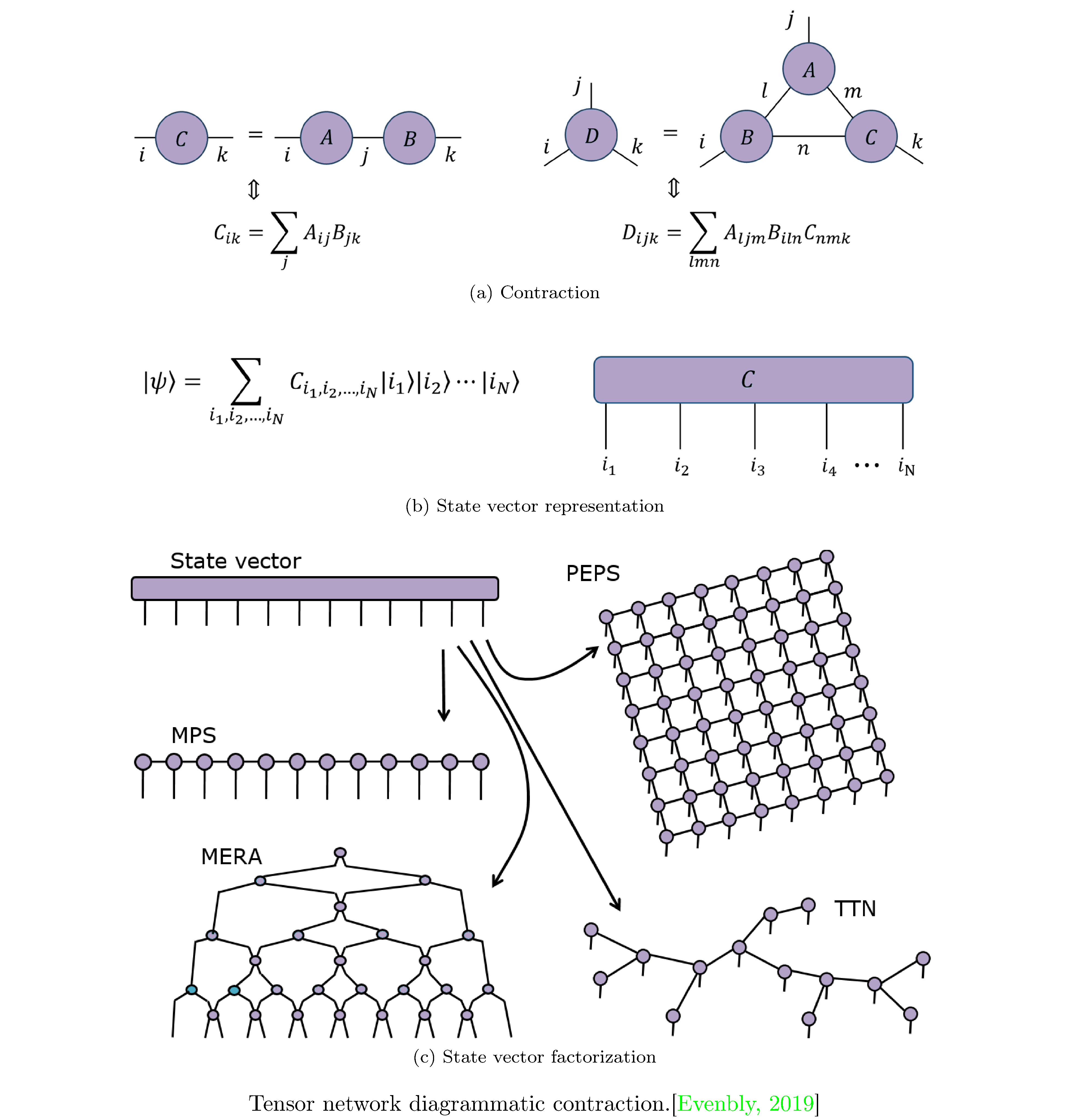
Tensor networks (TNs) are a way to factor tensors with large orders into networks of tensors with lower orders; since the number of parameters a tensor consists of is exponential in the order of the tensor, smaller order tensors are much preferable computationally. They were first used to study ground states of one dimensional quantum many-body systems [13] but have since been applied in other areas (such as machine learning [14]). TNs lend themselves to a diagrammatic representation which can be used to reason about such factorizations (figure 2). We will primarily be interested in TNs as a means to factoring the state-vector of an $N$-qubit system (see figure 2)
\[\ket{\psi}:=\sum_{i_{1}i_{2}\dots i_{N}}C^{i_{1}i_{2}\dots i_{N}}\ket{i_{1}}\ket{i_{2}}\cdots\ket{i_{N}}\label{eq:state_vector}\]for which its common to propose an ansatz factorizations:
-
Matrix Product States (MPS) [15], which yields factorization
\[C^{i_{1}i_{2}\dots i_{N}}\equiv A_{j_{1}}^{i_{1}}A_{j_{2}}^{i_{1}j_{1}}\cdots A_{j_{N-1}}^{i_{N-1}j_{N-2}}A^{i_{N}j_{N-1}}\]where $j$ are called bond indices. If each index $i$ has dimension $d$ (i.e. takes on values 1 to $d$) then $C$ is specified by $d^{N}$ parameters and can always be represented by an MPS factorization $Ndm^{2}$ parameters, where $m:=d^{N/2}$ is the bond dimension. While for this naive representation $d^{N}<Ndm^{2}$, in practice $m$ is fixed to some moderate size such that $d^{N}>Ndm^{2}$ and the MPS factorization functions as an approximation.
-
Projected Entangled Pair States (PEPS) [16], which is a generalization of MPS to higher spatial dimensions, i.e. TNs that correspond to lattices of contractions of tensors, which themselves represent pairwise entangled quantum systems. Naturally, such a series of contractions doesn’t lend itself to being expressed in traditional notation and thus we observe the power of tensor network diagrams (see PEPS in figure 2).
-
Tree Tensor Networks (TTN) [17], a further generalization where tensors are entangled (and therefore contracted) hierarchically. In fact TTNs bear the closest resemblance to quantum circuits.
-
Multi-scale Entanglement Renormalization Ansatz (MERA) [18], a specific type of TTN where the tensors are alternatingly unitaries and isometries11.
TNs for Simulating Quantum Circuits
Factoring eqn. $\eqref{eq:state_vector}$ is only the first step to successfully simulating a quantum circuit. By representing some final state as a tensor as well, and contracting across all indices (called contracting the network), we can calculate the amplitude for that particular state. Since tensor contraction is associative12, the order in which tensors are actually contracted is a “hyper-parameter” of TN methods; finding the optimal contraction order, with respect to accuracy (assuming some approximation has been made in constructing the factorization), compute time, and memory requirements is critical.
In particular we focus on contraction orders for TTNs as they most closely resemble quantum circuits. For a TTN consisting of $N$ tensors (corresponding to $N$ gates) with maximum order $p$, worst case, we can see that contraction time takes $O\left(N\exp\left(O\left(p\right)\right)\right)$ since, in general, contracting across all indices of a pair of tensors is exponential in their orders13. Markov et al. [19] showed that there in fact exists a contraction ordering which results in a contraction time of $O\left(N^{O\left(1\right)}\exp\left(O\left(\operatorname{tw}\left(G^{L}\right)\right)\right)\right)$ where $G^{L}$ is the line graph14 of the tensor network and $\operatorname{tw}\left(G^{L}\right)$ is the tree-width15 of $G^{L}$.
For quantum circuits consisting of many few qubit gates this technique produces a much more (runtime) efficient evaluation of the circuit; indeed Markov et al. further show that any TTN corresponding to a quantum circuit with $N$ gates, where the number of gates that act on any pair of qubits is bounded by $r$, has contraction time $O\left(N^{O\left(1\right)}\exp\left(O\left(r\right)\right)\right)$.
Markov et al.’s results are not tight; their construction finds some tree-decomposition with the correct corresponding tensor contraction order that suits their aim (overall runtime complexity of the translation from quantum circuit to TTN and the ultimate contraction). In reality there are often contraction orders that are much more space and runtime efficient. Though, in general problem is NP-hard [20], for particular TTNs (corresponding to circuits) there are heuristics, such as non-adjacent contractions [7], that produce more efficient orders. Alternatively, randomized search and Bayesian optimization can be used to identify efficient contraction orders [8, 21].
FPGAs
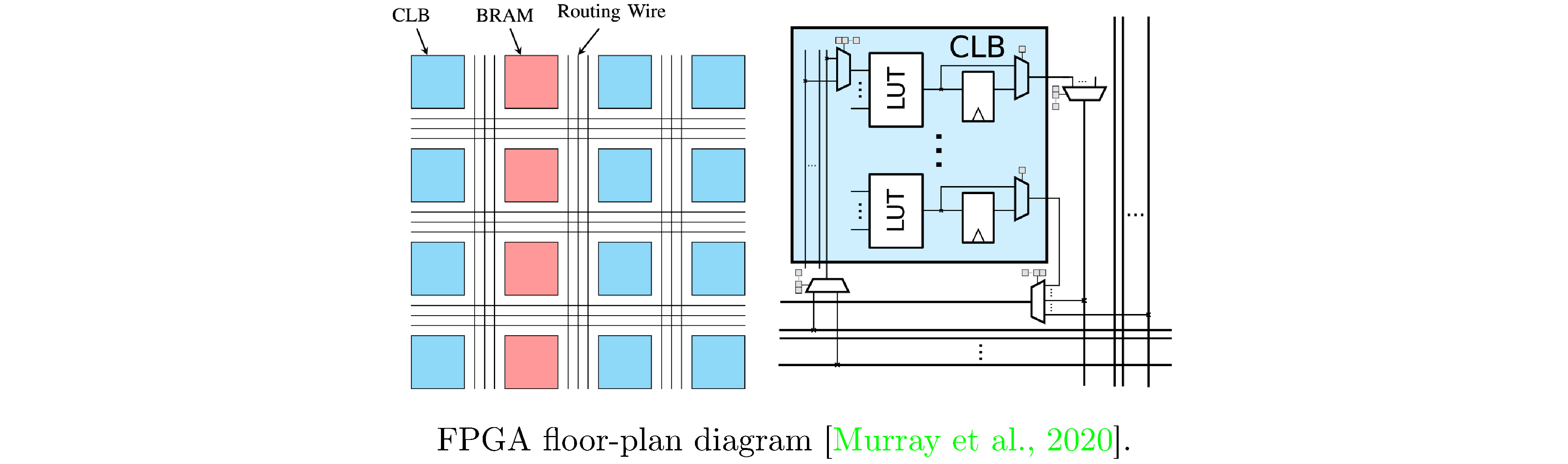
A field-programmable gate array (FPGA) is a device designed to be configured by a user into various arrangements of (classical) gates and memory. FPGAs consist of arrays (hence the name) of configurable logic blocks (CLBs), static ram (SRAM), and programmable busses that connect CLBs and SRAM into various topologies (see figure 3). The CLBs typically contain arithmetic units (such as adders, multipliers, and accumulators) and lookup tables (LUTs), that can be programmed to represent truth tables for many boolean functions. Using hardware description languages (such as VHDL or Verilog) designers specify modules and compose them into circuits (also known as data-flows) that perform arbitrary computation. These circuits then go through a place and route procedure before ultimately being instantiated on the FPGA as processing elements (PEs) and connections between PEs.
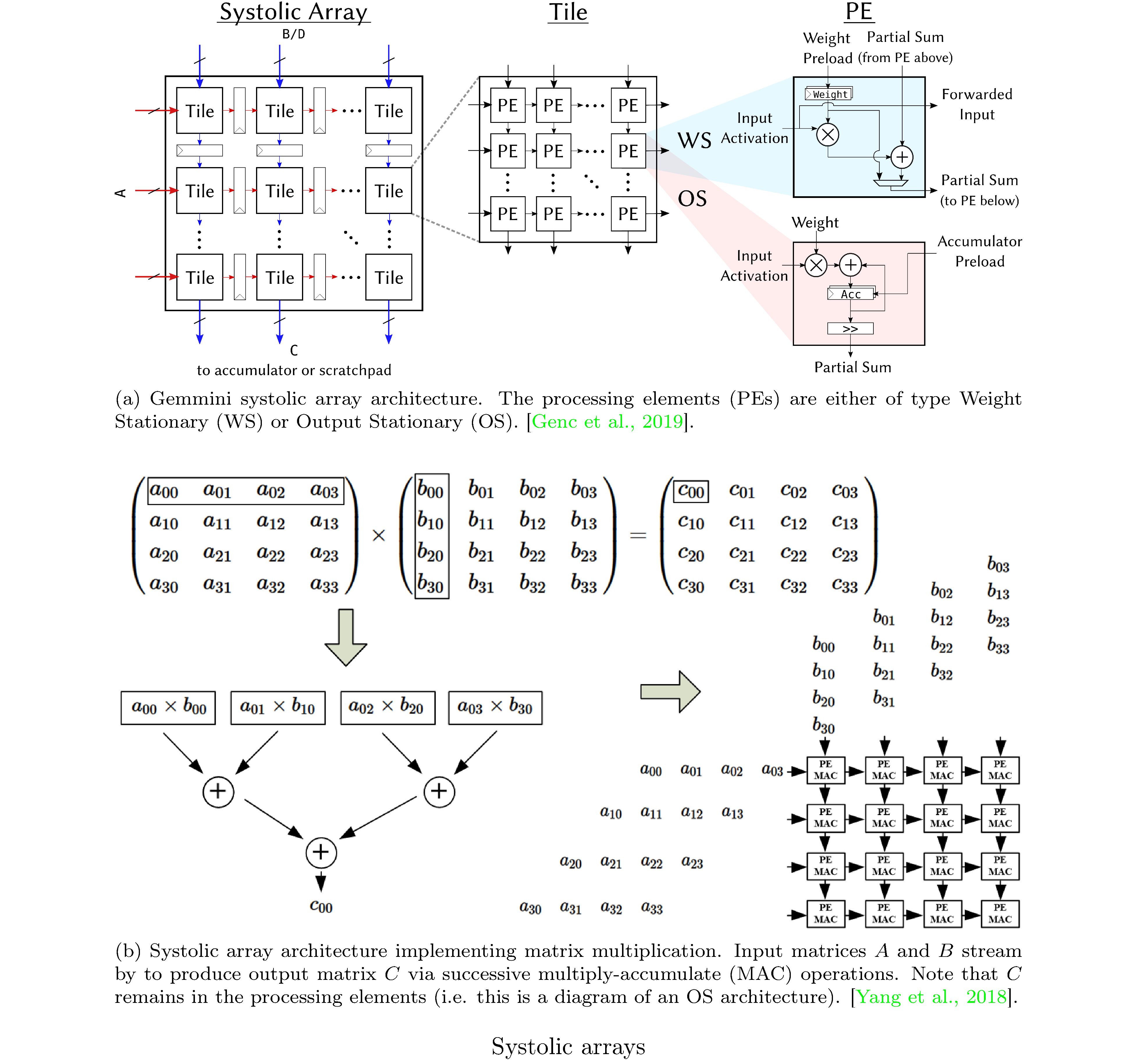
While modules consisting purely of combinational logic compute their outputs at the stated clock speed of the FPGA, inevitably I/O (i.e. fetching data from memory) interleaved with such modules (otherwise arranged into a pipeline architecture) creates pipeline stalls. Thus, it’s essential that FPGA designs are as compute bound as possible (rather than I/O bound). In particular, we explore I/O minimal generalized matrix multiplication (GEMM) [22] and other systolic array architectures [23, 24]. A systolic architecture [25] is a gridded, pipelined, array of PEs that processes data as the data flows16 through the array. Crucially, a systolic architecture propagates partial results as well as input data through the pipeline (see figure 4). Systolic arrays are particularly suited for I/O efficient matrix multiplication owing to the pipelining of inputs (see figure 4).
One remaining hurdle to simulating quantum computations (i.e. carrying out tensor contractions) on FPGAs is SRAM. The standard remediation is to perform arithmetic with reduced precision17. There is evidence that suggests that simulations of quantum circuits, of varying depths [26], are robust to reduced precision computation as long as that loss of precision is uncorrelated [27] i.e. insofar as it can be treated as uncorrelated noise.
Implementation
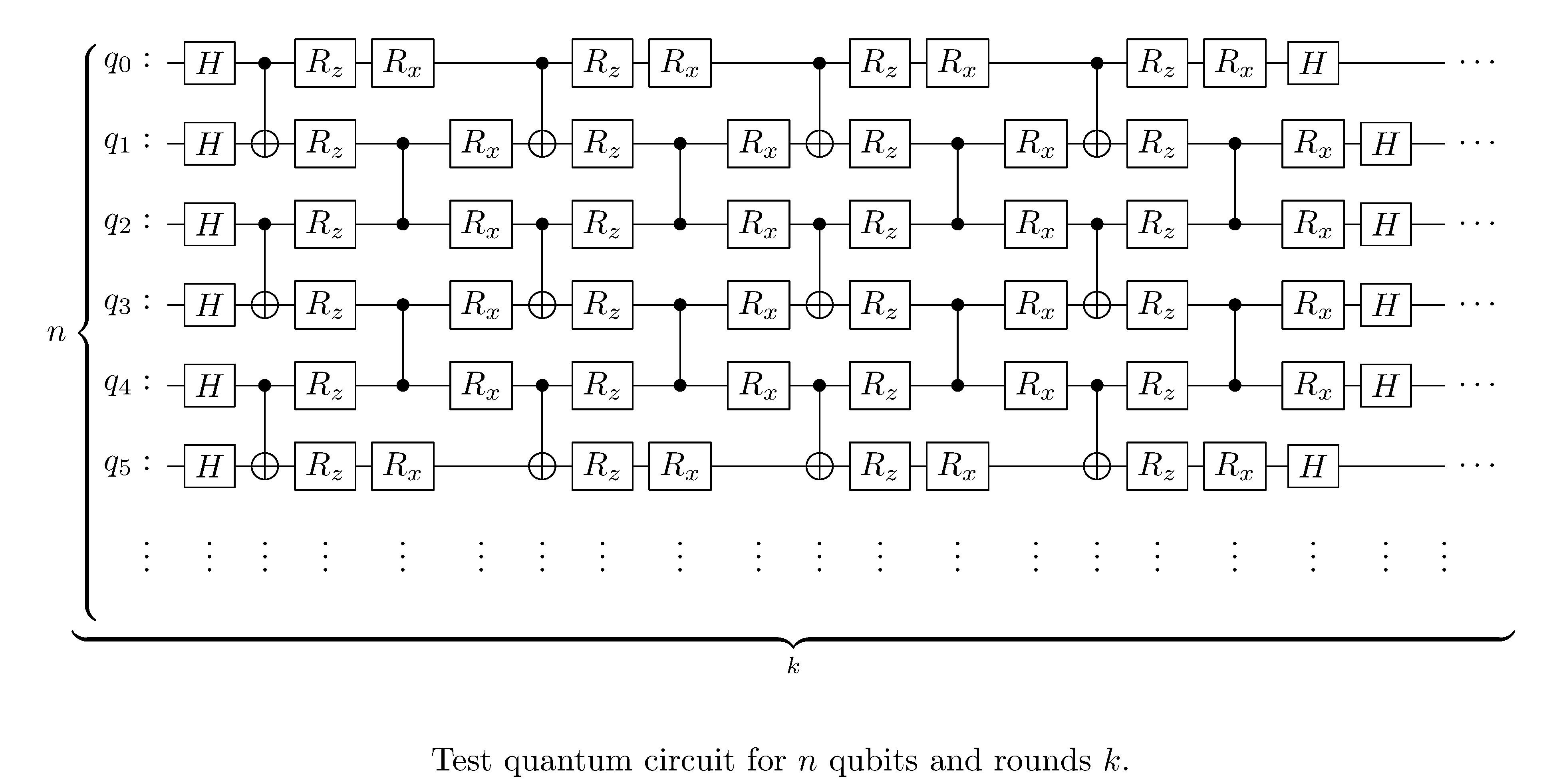
We use quimb [28] to specify quantum circuits and
generate TNs therefrom. In particular we simulate circuits for various
$n$ qubits and rounds $k$, where each consists of alternating qubit
couplings of the form in figure
5.
We also use Bayesian parameter optimization (BPO)
[21] to find tensor contraction orders and compare
against naive greedy search. Note that for both strategy we set a
timeout of 600 seconds. We then deploy the contraction strategy that
produces the fewest number of tensor contractions balanced against the
orders of intermediate tensors18. In order to expedite the process of
deploying we precompute some first few tensor contraction such that all
tensors deployed to the FPGA are square and congruent (i.e. all of the
same dimensions). For tensors of order greater than $\left(1,1\right)$
(i.e. tensors that are not matrices) we transform them into
$\left(1,1\right)$ tensors by taking the Kronecker product of all
component $\left(1,1\right)$ tensors; to be precise we perform the
following operation on the $\left(p,q\right)$ order tensor t
mats = [t[idx] for idx in np.ndindex(t.shape[:-2])]
    block_mat = block_diag(*qubit_mats)
where block_diag builds a block diagonal matrix of its arguments. All
of our code has been made available on GitHub19.
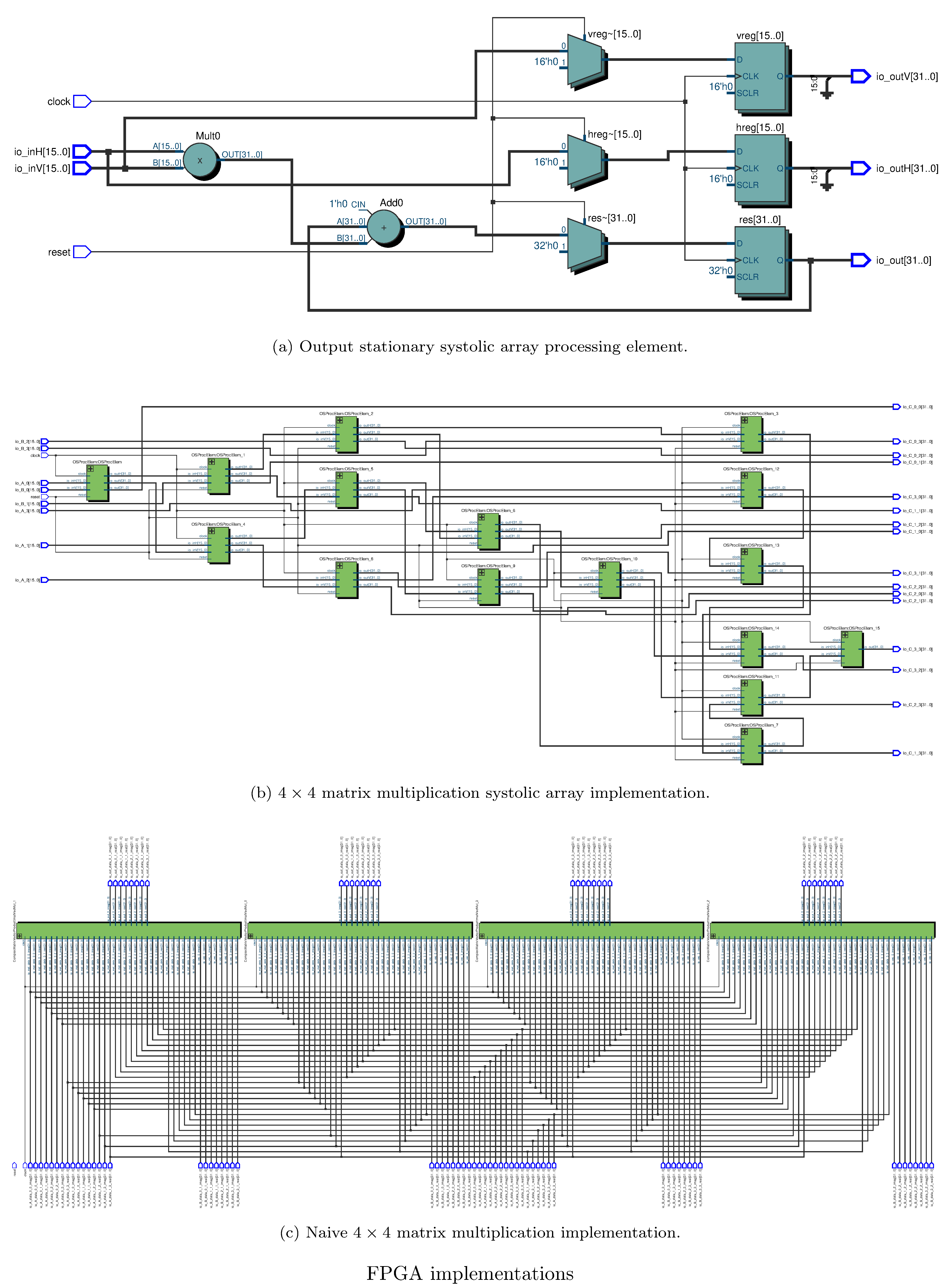
For defining FPGA circuits we use Chisel [29] as a HDL, by way of an adaptation of the Gemmini systolic array generator [24]. Notably we experiment with using Gemmini as an accelerator (i.e. fully parameterizing the weights/entries of the matrices) and “hardcoding” certain gates/tensors, i.e. naive matrix mutiplication. One possible advantage of the latter approach over the former is a reduction in loads from memory for the weights. The success of either approach depends heavily on whether certain sequences of fixed gates can actually be pipelined or alternatively deployed in toto to the FPGA. We hypothesize that this might depend on the depth and gate count of the circuits/TNs. See figure 6 for the netlists corresponding to our systolic array and naive matrix multiplication circuit implementations. Note that all (complex) arithmetic was done in 32 bit fixed precision for both implementations, with 28 bits allocated behind the binary point.
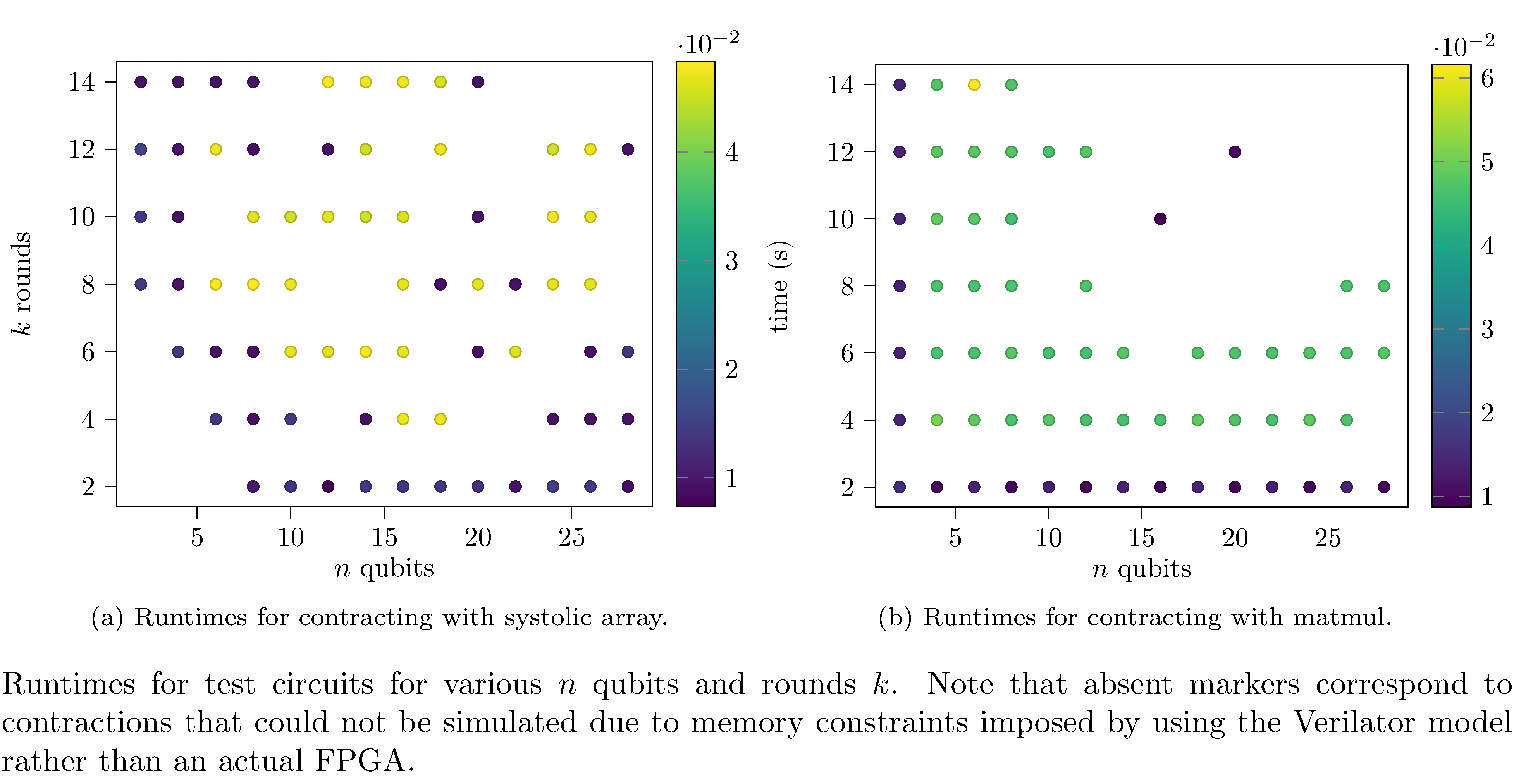
One challenge we faced was in deploying to real hardware20; unfortunately time and administrative challenges21 prevented us from actually deploying to real FPGAs. As a substitute we used the well-known and trusted Verilog simulator22 Verilator23, which transpiles Verilog (which Chisel generates) to a cycle-accurate model in C++. We then executed this cycle-accurate model to collect proxy measurements. Note that for certain configurations (generally those with high qubit and round count) we could not successfully simulate due to memory constraints on the workstation running the Verilator produced model.
Evaluation
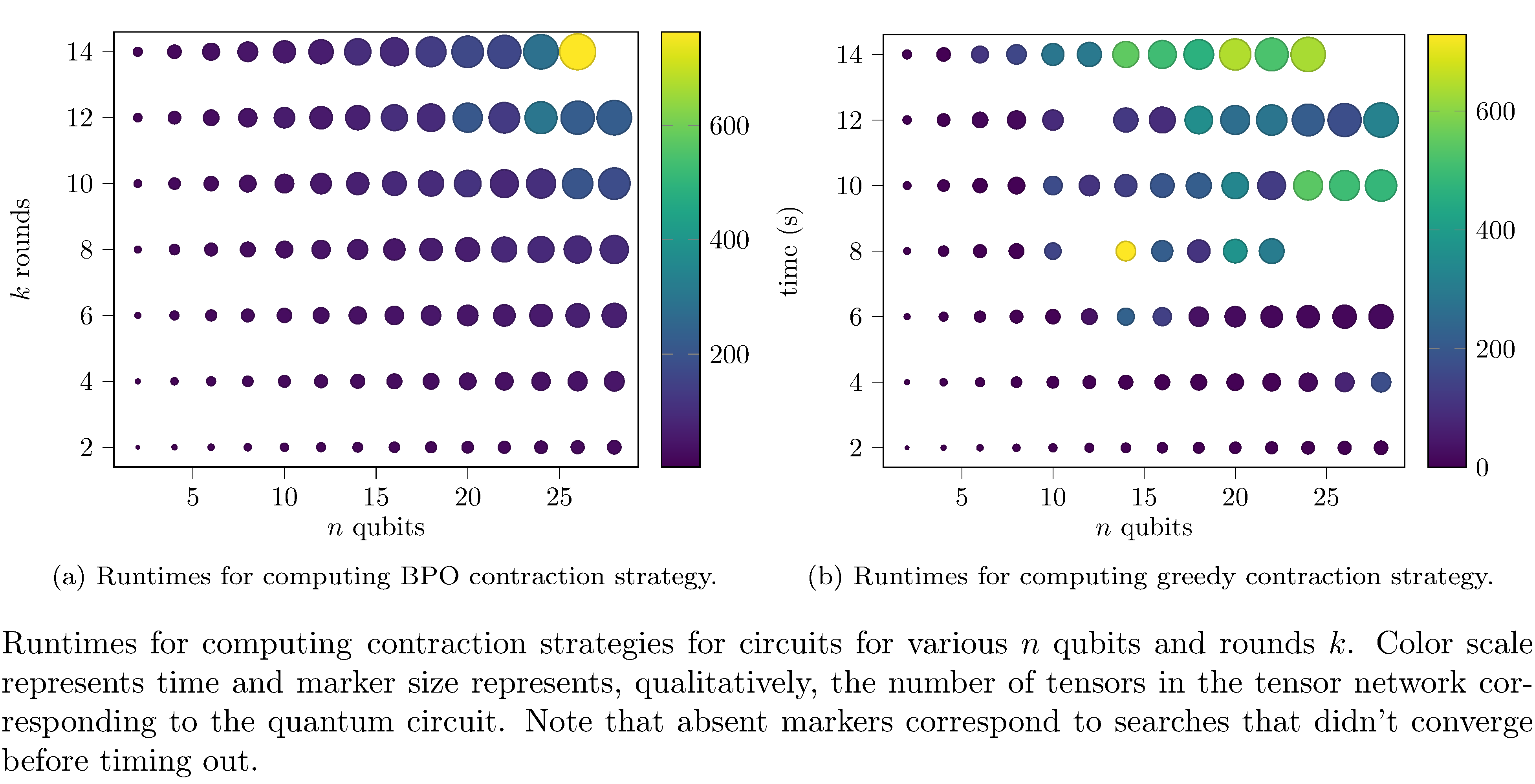
We perform two sets of evaluations. Even though it was not the central goal of our exploration, we first compare the time required to compute a tensor contraction strategy across $n$ qubits and rounds $k$ for the greedy search strategy and the BPO search strategy. We then addressed our central goal by comparing the actual runtime for performing the discovered tensor contraction on both the systolic array implementation (see fig. 6) and the “hardcoded” naive matrix multiplication implementation (see fig. 6).
Some interesting things to note regarding searching for contractions: computing (not evaluating) the optimal contraction strategy (i.e. using BPO) is generally more performant that greedy search (see figures 7, 7). The likely reason for this is that BPO converges more quickly and more efficiently searches the space of possible contraction orders than greedy search (which greedily optimizes some surrogate objective). Also note that, in fact, for certain configurations greedy didn’t even converge within the timeout.
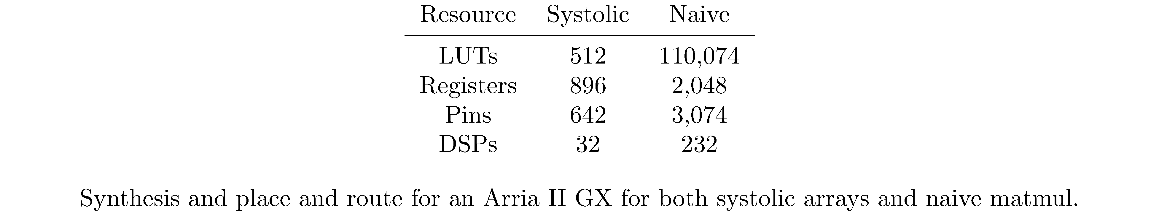
Regarding the differences in the evaluation times of the contraction orders (figures 8, 8) it’s clear that the systolic array implementation performs better in terms of both memory requirements and runtime. This is paradoxically both obvious and surprising. As already mentioned, one expects systolic arrays to have improved performance relative to naive matrix multiplication for streaming data (and indeed, in general, they do) but for this use case (where all matrix elements are known at deploy time) one also expects that latency incurred by pipelining would offset that performance improvement. One hypothesis for this is that the difference is an artifact of simulating the FPGA implementations insofar as simulating a more densely connected FPGA implementation (see the differences between 6 and 6) is more compute intensive, especially with respect to heap allocations (since systolic arrays incur more loads from memory). To corroborate this hypothesis we used Intel’s Quartus EDA24 tool to synthesize and place and route (for an Arria II GX). Indeed the naive implementation consumes an order of magnitude (and sometimes several) more of each type of resource (see table 1).
Conclusion
We explored tensor networks deployed to FPGAs as a means of accelerating simulations of quantum circuits. In order to accomplish this goal we expressed tensor contraction as sequences of matrix multiplications and implemented two different matrix multiplication FPGA designs: systolic arrays, which operate on streaming matrix elements and naive matrix multiplication, which wholecloth instantiates all the necessary MAC operations. In order to choose the contraction orders we used an “off the shelf” library which searches for a suitable contraction by either performing greedy search or Bayesian optimization. We compared the performance of both the contraction search strategy and each contraction evaluation implementation. Unfortunately we were unable to obtain access to FPGA devices and thus we made do with cycle-accurate simulations. Results for both comparison were generally in agreement with intuition: BPO converged to a contraction order more effectively (more quickly and more robustly) than greedy search and systolic arrays evaluated the contractions more efficiently than naive matrix multiplication.
Possible future work includes actually deploying to real FPGAs and then further comparing performance to the simulations performed here. Another particularly interesting research direction is the tangential problem of discovering optimal tensor contraction orders. Finding such tensor contraction orders is ultimately a combinatorial optimization problem. It occurs to us that possibly a deep learning approach could be effective. Recently there has been work on reinforcement learning for combinatorial optimization [30] and monte-carlo tree-search for combinatorial optimization [31] that could, possibly, be adapted to this problem in a straightforward fashion.
References
Footnotes
-
A Hilbert space $H$ is a vector space augmented with an inner product such that, with respect to the metric induced by that inner product, all Cauchy sequences converge. ↩
-
We say that the qubit is in a superposition of the basis vectors/states. ↩
-
$\xi$ cannot be factored because there is no solution to the set of equations (for $\alpha,\alpha’,\beta,\beta’$)
\[\alpha\alpha'=\frac{1}{\sqrt{2}},\quad\alpha\beta'=0,\quad\beta\alpha'=0,\quad\beta\beta'=\frac{1}{\sqrt{2}}\] -
A matrix $U$ is unitary iff $UU^{\dagger}=U^{\dagger}U=I$, i.e. it is its own Hermitian conjugate or more simply if it is “self-inverse.” ↩
-
The output of a combinational logic circuit at any time is only a function of the elements of the circuit and its inputs. ↩
-
There are several more at varying levels of mathematical sophistication. Chapter 14 of [12] is the standard reference. Ironically, it is this author’s opinion that one should shy away from physics oriented expositions on tensors. ↩
-
The collection of tensor products of elements of the component spaces quotiented by an equivalence relation. ↩
-
The dual space to a vector space $V$ is the vector $V^{*}$ consisting of linear maps $f:V\rightarrow\mathbb{R}$. The dual basis of the dual space consists of $f_{i}$ such that \(f_{i}\left(\mathbf{e}_{i}\right)=\delta_{ij}\). It is convention to write $f_{i}$ as $\mathbf{e}^{i}$ (note the superscript index). ↩
-
The rank of a tensor is the minimum number of distinct basis tensors necessary to define it; the tensor in eqn. $\eqref{eq:tensor_coord}$ is in fact a rank 1 tensor. The definition is a generalization of the rank of a matrix (which, recalling, is the dimension of its column space, i.e. number of basis elements). Despite this obvious, reasonable definition for rank, one should be aware that almost all literature in this area of research uses rank to mean order. ↩
-
Repeated indices in juxtapose position indicate summation $a_{i}b^{i}:=\sum_{i}a[i]b[i]$. ↩
-
A tensor, seen as a multilinear map, that preserves distances under the ambient distance metric. ↩
-
This can be observed by noting that summing is an associative operation (or by analog with matrix-matrix multiplication). ↩
-
Consider contracting two $\left(1,1\right)$ tensors (as in eqn. $\eqref{eq:matrix_mult}$), i.e. two order 2 tensors, which effectively is matrix multiplication followed by trace. The complexity of this contraction is then $O\left(N^{2+1}+N\right)\equiv O\left(\exp\left(2\log N\right)\left(1+N\right)\right)$ (where $N$ here is the characteristic dimension of the matrix). Assuming the ranges of all tensor indices is the same (i.e. $N$ is constant across all tensors), for example $N=2$ as in the case of matrices derived of unitary transformations operating on single qubits, we recover the stated complexity. ↩
-
A line graph captures edge adjacency; given a graph $G$, $G^{L}$ is defined such that each edge of $G$ corresponds to a vertex of $G^{L}$ and two vertices are are connected in $G^{L}$ if the edges in $G$ that they correspond to are adjacent on the same vertex (in $G$). ↩
-
A tree decomposition of a graph $G$ is a tree $T$ and a mapping from the vertices of $G$ into “bags” that satisfy the following properties
-
Each vertex must appear in at least one bag.
-
For each edge in $G$, at least one bag must contain both of the vertices it is adjacent on.
-
All bags containing a given vertex in $G$ must be connected in $T$.
The width $w$ of a tree decomposition is the cardinality of the largest bag (minus one). Finally the tree-width of $G$ is the minimum width over all possible tree decompositions. Intuitively, a graph has low tree-width if it can be constructed by joining small graphs together into a tree. ↩
-
-
The relationship to cardiovascular “systolic” is in association with the flow of data into the array, akin to how blood flows through the veins into the human heart. ↩
-
Germaine to this issue is the fact that arithmetic on FPGAs is typically performed in fixed precision, owing to higher compute cost incurred for floating point arithmetic. ↩
-
This choice was purely due to platform constraints in that large intermediate tensors could not be effectively simulated. ↩
-
https://github.com/makslevental/fpga_stuff/ on the
complexmatmulbranch. ↩ -
A challenge not unfamiliar to the seasoned QC researcher. ↩
-
We were not able to get allocations on CHI@TACC in a timely fashion (the issue is ongoing…). ↩
-
It is simulations all the way down. ↩
-
Electronic design automation. ↩