
Towards Online Steering of Flame Spray Pyrolysis Nanoparticle Synthesis
- Introduction
- Flame Spray Pyrolysis
- Blob detection background
- Blob Detector Implementation
- Evaluation
- Related work
- Conclusion
- References
Flame Spray Pyrolysis (FSP) is a manufacturing technique to mass produce engineered nanoparticles for applications in catalysis, energy materials, composites, and more. FSP instruments are highly dependent on a number of adjustable parameters, including fuel injection rate, fuel-oxygen mixtures, and temperature, which can greatly affect the quality, quantity, and properties of the yielded nanoparticles. Optimizing FSP synthesis requires monitoring, analyzing, characterizing, and modifying experimental conditions. Here, we propose a hybrid CPU-GPU Difference of Gaussians (DoG) method for characterizing the volume distribution of unburnt solution, so as to enable near-real-time optimization and steering of FSP experiments. Comparisons against standard implementations show our method to be an order of magnitude more efficient. This surrogate signal can be deployed as a component of an online end-to-end pipeline that maximizes the synthesis yield.
Introduction
Flame Spray Pyrolysis (FSP) is used to manufacture nanomaterials employed in the production of various industrial materials. A FSP instrument rapidly produces nanoparticle precursors by combusting liquid dissolved in an organic solvent. Optical and spectrometry instrumentation can be used in a FSP experiment to monitor both flame and products. This provides insight into the current state and stability of the flame, quantity of fuel successfully combusted, and quantity and quality of materials produced. To avoid fuel wastage and to maximize outputs, data must not only be collected but also analyzed and acted upon continuously during an experiment.
A key technique for monitoring and determining a FSP experiment’s effectiveness is quantifying and classifying the fuel that is not successfully combusted. Planar Laser-Induced Fluoroscopy (PLIF) and optical imagery of the flame can be used to make informed decisions about an experiment and guide the fuel mixtures, fuel-oxygen rates, and various pressures. Fuel wastage can be approximated by detecting and quantifying the droplets of fuel that have not been successfully aerosolized (thus, uncombusted). Blob detection algorithms provide an effective means for both detecting fuel droplets and determining their sizes. Blob detection is the identification and characterization of regions in an image that are distinct from adjacent regions and for which certain properties are either constant or approximately constant. Note, however, that the volume and rate of the data generated by FSP instruments requires both automation and high-performance computing (HPC); the primary latency constraint is imposed by the collection frequency of the imaging sensor (ranging from 10Hz-100Hz).
Argonne National Laboratory’s Combustion Synthesis Research Facility (CSRF) operates a FSP experiment that produces silica, metallic, oxide and alloy powders or particulate films. However, standard processing methods on CPUs far exceeds FSP edge computing capacity, i.e. performing image analysis on the FSP device is infeasible. To address this need for rapid, online analysis we present a hybrid CPU-GPU method to rapidly evaluate the volume distribution of unburnt fuel.
Surrogate models can be employed to steer experiments by producing an inference for a quantity of interest faster than physical measurements [1]. In particular, machine learning surrogate models have been used in materials science, with varying degrees of success [2]. Here we aim to drive a Bayesian hyper-parameter optimizer (BO) that optimizes the various parameters of CSRF’s FSP experiment. The combination of FSP, our technique, and the BO, define an “end-to-end” system for optimizing FSP synthesis (see figure 1).

We integrate our solution into the Manufacturing Data and Machine Learning platform [3], enabling near-real-time optimization and steering of FSP experiments through online analysis.
The remainder of this paper is as follows: Section science discusses the materials science of FSP, Section blobdetection discusses blob detection and derives some important mathematical relationships, Section implementation covers practical considerations and our improvements to blob detection, Section evaluation compares our improved algorithms against standard implementations, Section related discusses related work, and Section conclusion concludes.
Flame Spray Pyrolysis
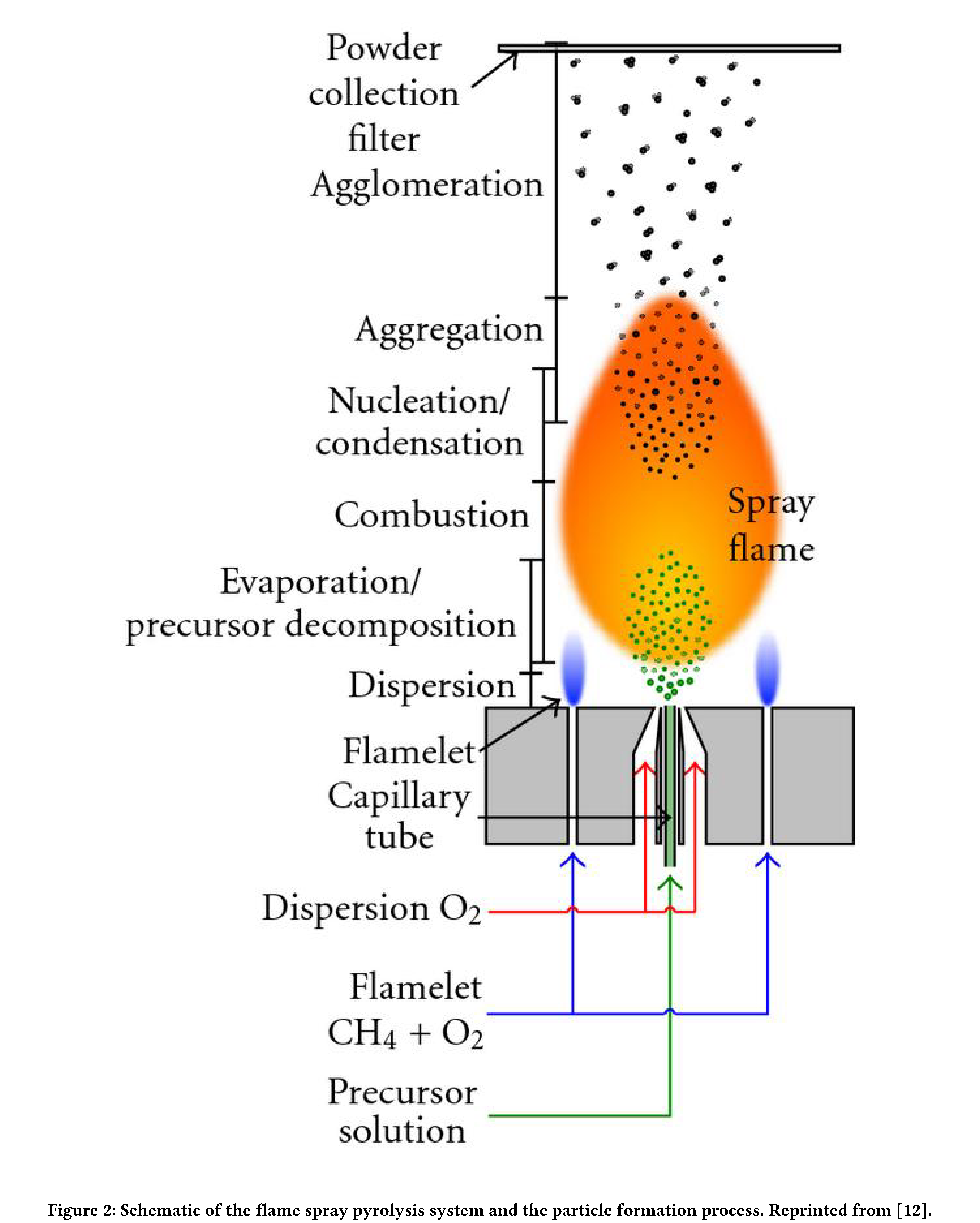
Flame aerosol synthesis (FAS) is the formation of fine particles from flame gases [4]. Pyrolysis (also thermolysis) is the separation of materials at elevated temperatures in an inert environment (that is, without oxidation). Flame Spray Pyrolysis (FSP) is a type of FAS where the precursor for the combustion reaction is a high heat of combustion liquid dissolved in an organic solvent [5] ( see Figure 2). An early example of industrial manufacturing employing FSP was in the production of carbon black, used, for example, as a pigment and a reinforcing material in rubber products.
Optimizing FSP reaction yield is challenging; there are many instrument parameters (sheath O2, pilot CH4 and solution flow rates, solute concentration, and air gap) and salient physical measurements often have low resolution in time. Reaction yield can be inferred from the FSP droplet size distribution, with smaller droplets implying a more complete combustion. Unfortunately, the characterization of droplet distribution via, for example, Scanning Mobility Particle Sizer Spectrometry (SMPSS) has an analysis period of roughly ten seconds [6],
while other measurement techniques, such as Raman spectroscopy, require even longer collection periods. These measurement latencies prevent the use of such characterization techniques for adaptive control of the experiment and hence optimization of experiment parameters.
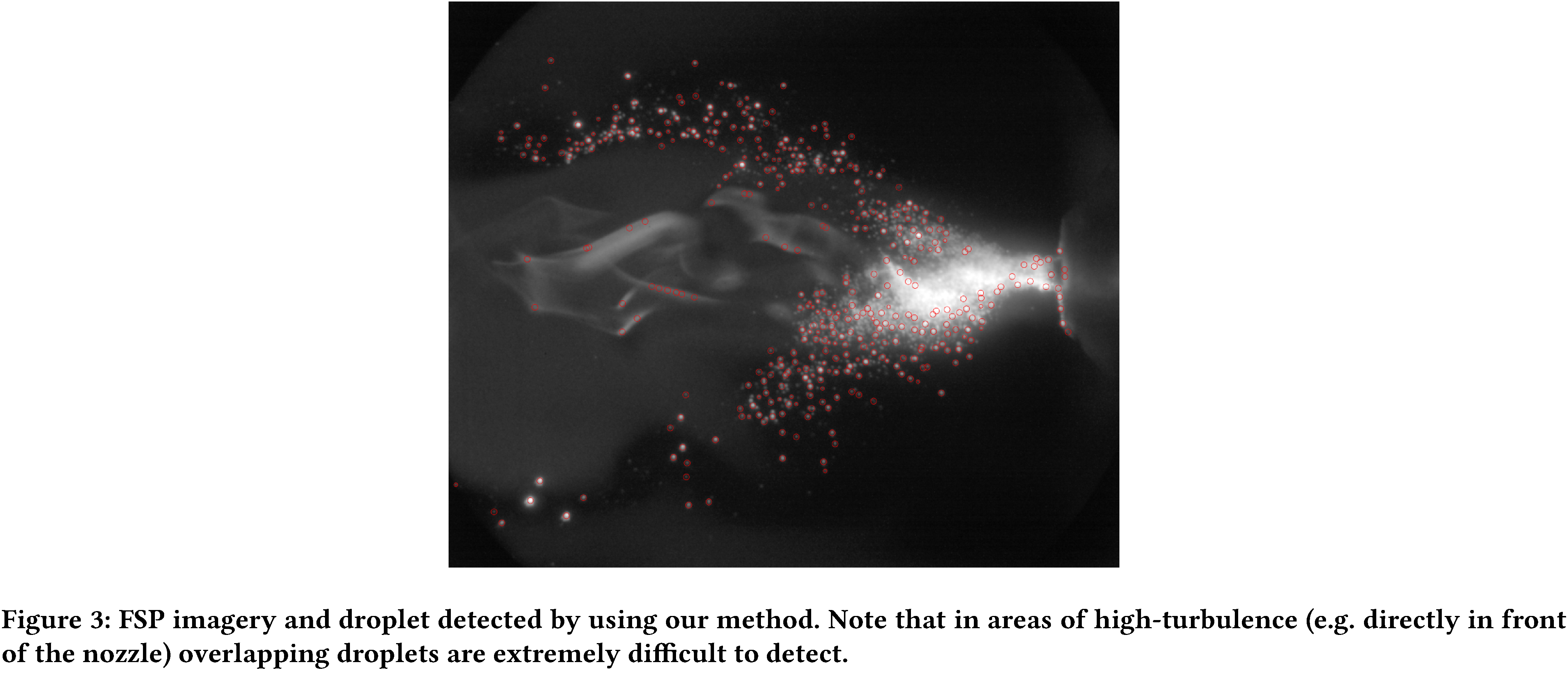
In this work, droplet imaging is performed by using a iSTAR sCMOS camera oriented perpendicular to a 285nm laser light sheet that bisects the flame along its cylindrical axis. Imagery is collected at 10Hz, with each image capturing the droplet distribution from a 10ns exposure due to the laser pulse. The images are formed by Mie scattering from the surfaces of the spherical droplets (see Figure 3). The image size is not calibrated to droplet size, and so we use relative size information to assess the atomization efficiency of the FSP.
Blob detection background
Blob detectors operate on scale-space representations [7]; define the scale-space representation $L(x,y,\sigma)$ of an image $I(x,y)$ to be the convolution of that image with a mean zero Gaussian kernel $g(x,y,\sigma)$, i.e.:
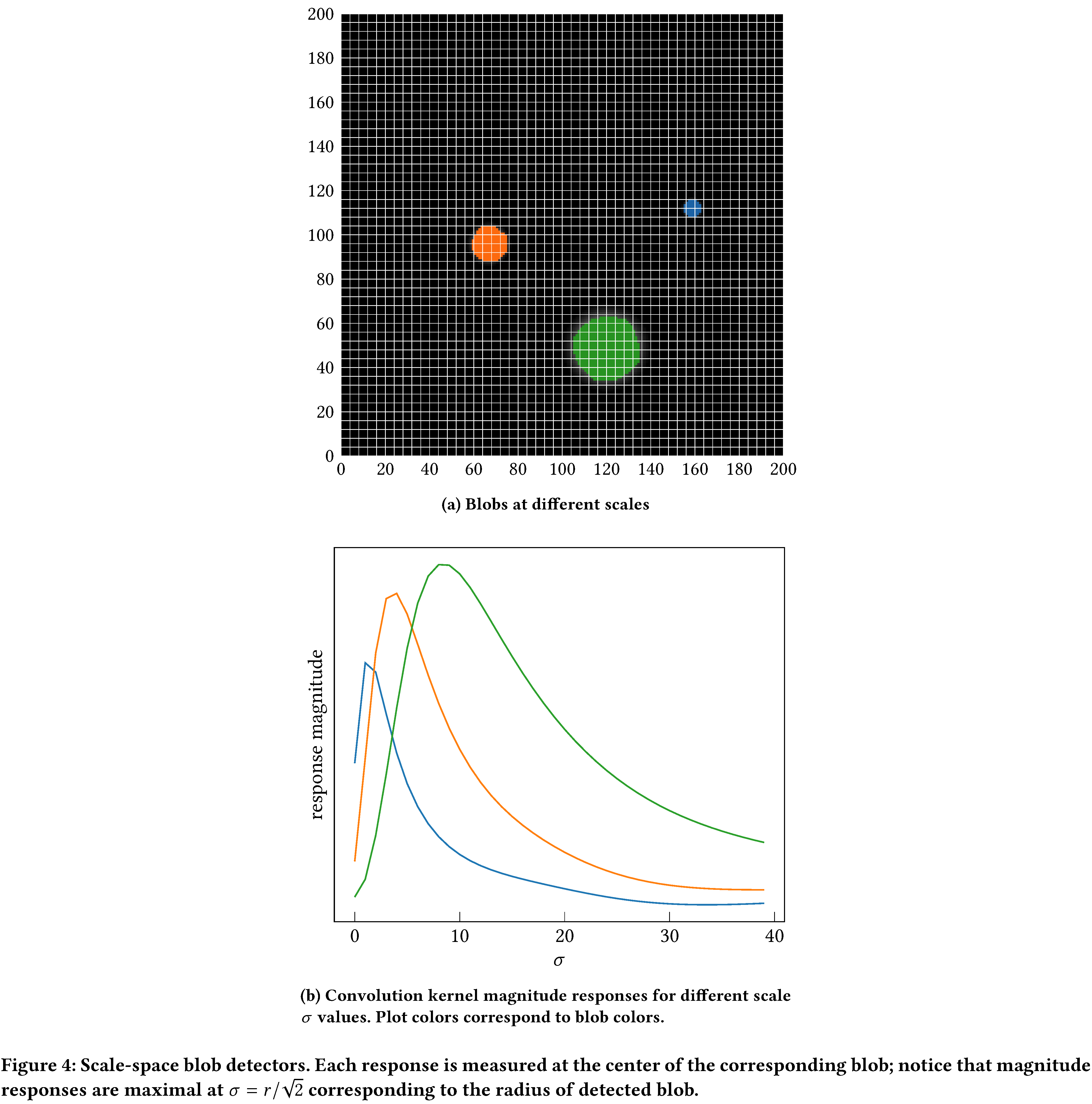
\[L(x,y,\sigma) \coloneqq g(x,y,\sigma) * I(x,y),\]where $\sigma$ is the standard deviation of the Gaussian and determines the scale of $L(x,y,\sigma)$. Scale-space blob detectors are also parameterized by the scale $\sigma$, such that their response is extremal when simultaneously in the vicinity of blobs and when $\sqrt{2}\sigma = r$ corresponds closely to the characteristic radius of the blob. In particular, they are locally extremal in space and globally extremal in scale, since at any given scale there might be many blobs in an image but each blob has a particular scale. Conventionally, scale-space blob detectors are strongly positive for dark blobs on light backgrounds and strongly negative for bright blobs on dark backgrounds. Two such operators are:
-
Scale-normalized trace of the Hessian:
\[\operatorname{trace}(H L) \coloneqq \sigma^2\left(\frac{\partial^2 L}{\partial x^2} + \frac{\partial^2 L}{\partial y^2}\right)\]Equivalently $\operatorname{trace}(H L) \coloneqq \sigma^2\Delta L$, where $\Delta$ is the Laplacian.
-
Scale-normalized Determinant of Hessian (DoH):
\[\operatorname{det} (H L) \coloneqq \sigma^4 \left(\frac{\partial^2 }{\partial x^2}\frac{\partial^2 L}{\partial y^2}-\left(\frac{\partial^2 L}{\partial x \partial y}\right)^2\right)\]
Note that by the associativity of convolution,
\[\sigma^2\Delta L = \sigma^2 \Delta \left(g * I\right) = \left( \sigma^2\Delta g \right) * I\]Consequently, $\sigma^2\Delta g$ is called the scale-normalized Laplacian of Gaussians (LoG) operator/blob detector.
DoH and LoG are both nonlinear (due to dependence on derivatives) and compute intensive (directly a function of the dimensions of the image), but in fact LoG can be approximated. Since $g$ is the Green’s function for the heat equation:
\[\begin{aligned} \sigma \Delta g &= \frac{\partial g}{\partial \sigma} \\ &\approx \frac{g(x,y,\sigma + \delta \sigma) - g(x,y,\sigma)}{\delta \sigma}\end{aligned}\]Hence, we see that for small, fixed, $\delta \sigma$
\[\sigma^2 \Delta g \approx \sigma \times [g(x,y,\sigma + \delta \sigma) - g(x,y,\sigma)]\]up to a constant. This approximation is called the Difference of Gaussians (DoG). In practice, one chooses $k$ standard deviations such that the $\sigma_i$ densely sample the range of possible blob radii, through the relation $\sqrt{2}\sigma_i = r_i$. For example, Figure 4 schematically demonstrates the response of a DoG detector that is responsive to approximately 40 blob radii, applied to three blobs.
While LoG is the most accurate detector, it is also slowest as it requires numerical approximations to second derivatives across the entire image. In practice, this amounts to convolving the image with second order edge filters, which have large sizes and thereby incur a large number of multiply–accumulate (MAC) operations. DoG, being an approximation, is faster than LoG, with similar accuracy. Hence, here we focus on LoG and derivations thereof.
Blob Detector Implementation
We abstractly describe a standard implementation of a blob detector that employs DoG operators, and then discuss optimizations.
A first, optional, step is to preprocess the images; a sample image (one for which we wish to detect blobs) is smoothed and then contrast stretched (with 0.35% saturation) to the range $[0,1]$. This preprocessing is primarily to make thresholding more robust (necessary for us because our imaging system has dynamic range and normalizes anew for every collection). Since DoG is an approximation of LoG, a sample image is first filtered by a set of mean zero Gaussian kernels ${g(x,y,\sigma_i)}$ in order to produce the set of scale-space representations ${L(x,y,\sigma_i)}$. The quantity and standard deviations of these kernels is determined by three hyperparameters:
-
n_bin— one less than the number of Gaussian kernels. This hyperparameter ultimately determines how many different radii the detector can recognize. -
min_sigma— proportional to the minimum blob radius recognized by the detector. -
max_sigma— proportional to the maximum blob radius recognized by the detector.
Therefore, define $\delta\sigma \coloneqq (\mathtt{max_sigma} - \mathtt{min_sigma})/\mathtt{n_bin}$ and
\[\sigma_i \coloneqq \mathtt{min\_sigma} + (i-1) \times \delta\sigma\]for $i=1, \dots, (\mathtt{n_bin}+1)$. This produces an arithmetic progression of kernel standard deviations such that $\sigma_1 = \mathtt{min_sigma}$ and $\sigma_{\mathtt{n_bin}} = \mathtt{max_sigma}$. Once an image has been filtered by the set of mean zero Gaussian kernels, we take adjacent pairwise differences
\[\Delta L_i \coloneqq L(x,y,\sigma_{i+1})-L(x,y,\sigma_i)\]for $i=1, \dots, \mathtt{n_bin}$, and define
\[\operatorname{DoG}(x,y,\sigma_i) \coloneqq \sigma_i \times \Delta L_i\]We then search for local maxima
\[\{(\hat{x}_j, \hat{y}_j, \hat{\sigma}_j)\} \coloneqq \operatorname*{argmaxlocal}_{x,y, \sigma_i} \operatorname{DoG}(x,y,\sigma_i)\]Such local maxima can be computed in various ways (for example, zero crossings of numerically computed derivatives) and completely characterize circular blob candidates with centers $(\hat{x}_j, \hat{y}_j)$ and radii $\hat{r}_j = \sqrt{2}\hat{\sigma}_j$. Finally blobs that overlap in excess of some predetermined, normalized, threshold can be pruned or coalesced. Upon completion, the collection of blob coordinates and radii ${(\hat{x}_j, \hat{y}_j, \hat{\sigma}_j)}$ can be transformed further (for example, histogramming to produce a volume distribution).
An immediate, algorithmic, optimization is with respect to detecting extrema. We use a simple heuristic to identify local extrema: for smooth functions, values that are equal to the extremum in a fixed neighborhood are in fact extrema. We implement this heuristic by applying an $n \times n$ maximum filter $\operatorname{Max}(n,n)$ (where $n$ corresponds to the neighborhood scale), to the data and comparing:
\[\operatorname*{argmaxlocal}_{x,y} I \equiv \{x,y \,| (\operatorname{Max}(n,n)*I - I) = 0 \}\]Second, note that since $\operatorname{DoG}(x,y,\sigma_i)$, in principle, is extremal for exactly one $\sigma_i$ (that which corresponds to the blob radius) we have
\[\operatorname*{argmaxlocal}_{x,y, \sigma_i} \operatorname{DoG}(x,y,\sigma_i) = \operatorname*{argmaxlocal}_{x,y} \operatorname*{argmax}_{\sigma_i} \operatorname{DoG}(x,y,\sigma_i)\]Thus, we can identify local maxima of $\operatorname{DoG}(x,y,\sigma_i)$ by the aforementioned heuristic, by applying a 3D maximum filter to the collection $\operatorname{Max}(n,n,n)$ to ${\operatorname{DoG}(x,y,\sigma_i)}$. Typically, neighborhood size is set to three. This has the twofold effect of comparing scales with only immediately adjacent neighboring scales and setting the minimum blob proximity to two pixels.
Further optimizations are implementation dependent. A reference sequential (CPU) implementation of the DoG blob detector is available in the popular Python image processing package scikit-image [8]. For our use case, near real-time optimization, this reference implementation was not performant for dense volume distributions (see Section evaluation). Thus, we developed a de novo implementation; the happily parallel structure of the algorithm naturally suggests itself to GPU implementation.
GPU Implementation
We use the PyTorch [9] package due its GPU primitives and ergonomic interface. Our code and documentation are available [10]. As we use PyTorch only for its GPU primitives, rather than for model training, our implementation consists of three units with “frozen” weights and a blob pruning subroutine.
We adopt the PyTorch
$\mathtt{C_{out}} \times \mathtt{H} \times \mathtt{W}$ convention for
convolution kernels and restrict ourselves to grayscale images. Hence,
the first unit in our architecture is a
(n_bin+1) \times max_width \times max_width 2D convolution, where
max_width is proportional to the maximum sigma of the Gaussians
(discussed presently). Note that the discretization mesh for these
kernels must be large enough to sample far into the tails of the
Gaussians. To this end, we parameterize this sampling
$\mathtt{radius}_i$ as
$\mathtt{radius}_i \coloneqq \mathtt{truncate} \times \sigma_i$ and
set $\mathtt{truncate} = 5$ by default (in effect sampling each Gaussian
out to five standard deviations). The width of each kernel is then
$\mathtt{width}_i \coloneqq 2\times\mathtt{radius}_i + 1$ in order
that the Gaussian is centered relative to the kernel. To compile this
convolution unit to a single CUDA kernel, as opposed to a sequence of
kernels, we pad with zeros all of the convolution kernels (except the
largest) to the same width as the largest such kernel. That is to say
The second unit is essentially a linear layer that performs the adjacent differencing and scaling discussed in Section implementation. The maximum filtering heuristic is implemented using a $3 \times 3 \times 3$ 3D maximum pooling layer with stride equal to 1 (so that the DoG response isn’t collapsed). Blobs are then identified and low confidence blobs (DoG response lower than some threshold, by default $0.1$) are rejected
\[\operatorname{Thresh}(x,y,\sigma) \coloneqq \begin{cases} 1 \text{ if } \left(\operatorname{MaxPool3D} * D - D = 0\right) \bigwedge (D > 0.1) \\ 0 \text{ otherwise} \end{cases}\]where $D \coloneqq D(x,y,\sigma)$. Once true blobs are identified, overlapping blobs can be pruned according to an overlap criterion; pruning proceeds by finding pairwise intersections amongst blobs and coalescing blobs (by averaging the radius) whose normalized overlap exceeds a threshold (by default $0.5$). Blobs are then histogrammed, with bin centers are equal to ${\hat{r}_i}$. Currently pruning and histogramming are both performed on the CPU but could be moved to the GPU as well [11, 12].
Surprisingly, for the naive PyTorch implementation of DoG there is a
strong dependence on max_sigma. This turns out to be due to how
convolutions are implemented in PyTorch. Further refining the GPU
implementation by implementing FFT convolutions sacrifices (slightly)
independence with respect to n_bin, but renders the detector constant
with respect to max_sigma and dramatically improves performance (see
Section evaluation).
Evaluation
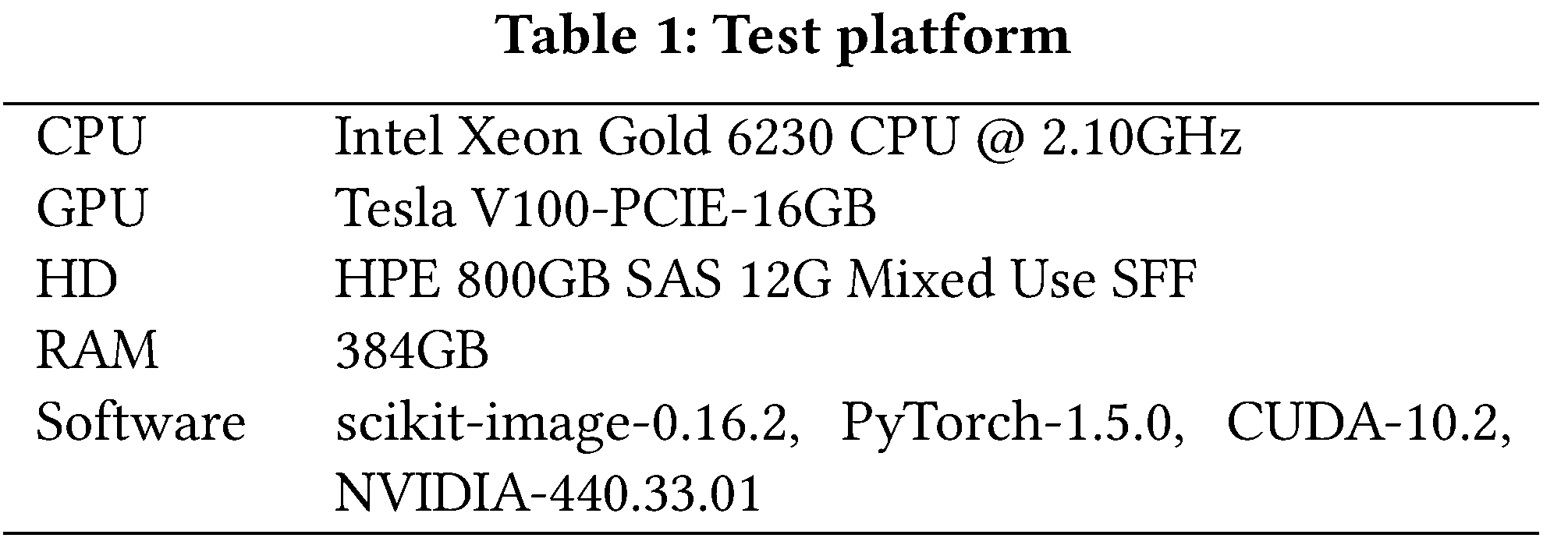
We compare our GPU implementation of DoG against the standard implementation found in scikit-image. Our test platform is described in Table 5. Both detectors were tested on simulated data generated by a process that emulates the FSP experiment; a graphics rendering engine renders 100 spheres and then Poisson and Gaussian noise [13] is added to the rendered image. The images have a resolution of 1000 $\times$ 1000 pixels. We turn off overlap pruning as it is the same across both methods (performed on the CPU). In order to perform an “apples to apples” comparison we exclude disk I/O and Host-GPU copy times from the charted measurements; we discuss the issue of Host-GPU copy time as potentially an inherent disadvantage of our GPU implementation in the forthcoming.
We compare precision and recall, according to PASCAL VOC 2012 [14] conventions, for both the CPU and GPU implementations. The precision and recall differences have means $-3.2 \times 10^{-4}, 3.5 \times 10^{-3}$ and standard deviations $4.0\times 10^{-6}, 2.0\times 10^{-4}$ respectively. This shows that for a strong majority of samples, the precision and recall for a given sample are exactly equal for both implementations; on rare occasions there is a difference in recall due to the padding of the Gaussian kernels for the GPU implementation.
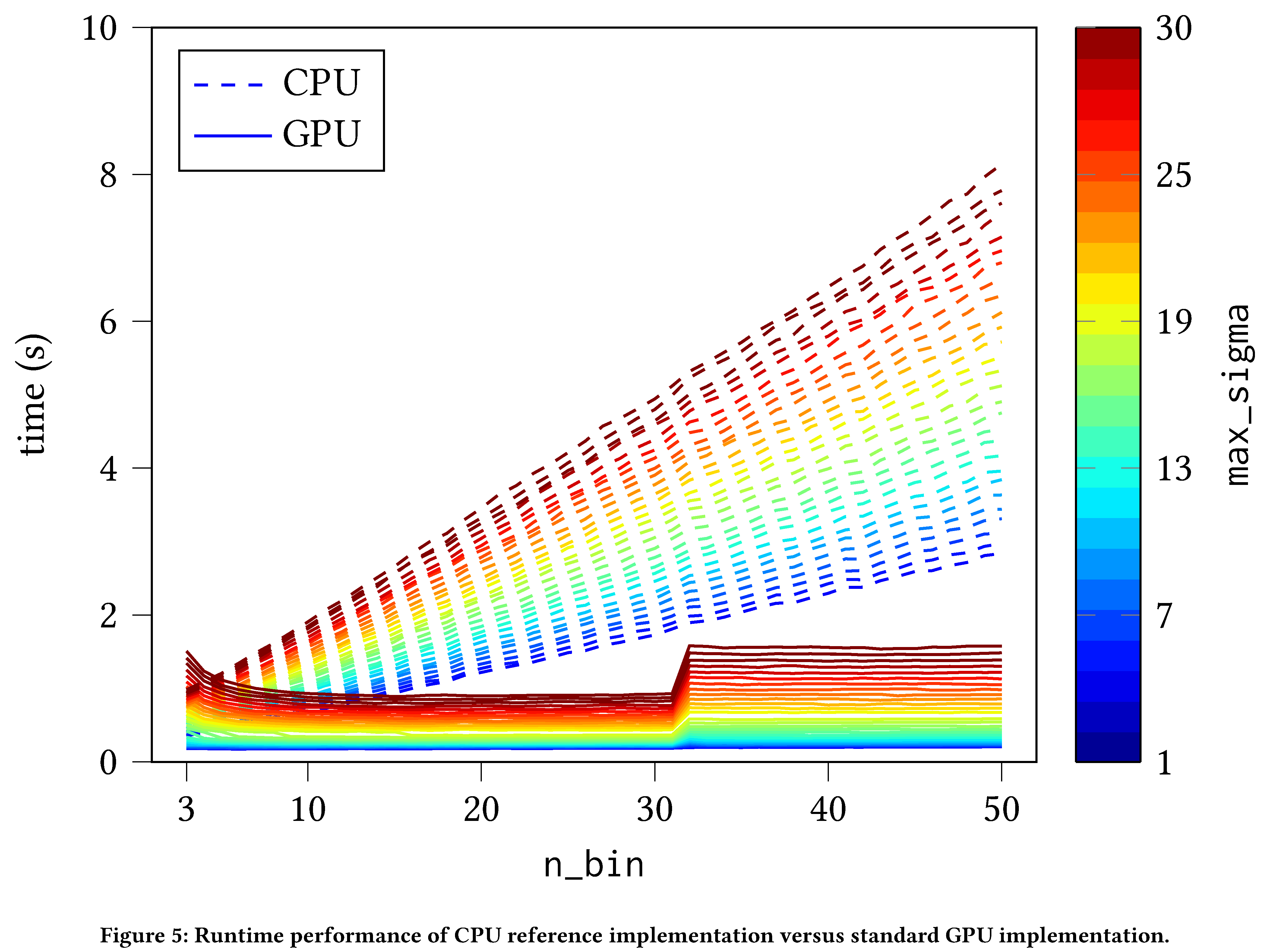
The performance improvement of the straightforward translation of the
standard algorithm to PyTorch is readily apparent. The PyTorch
implementation is approximately constant in n_bin (i.e. the number of
Gaussian filters) owing to the inherent parallelism of GPU compute (see
Figure 7)
while the CPU implementation scales linearly in n_bin (owing to the
sequential nature of execution on the CPU). We see a discontinuous
increase in runtime for the standard GPU implementation at
$\mathtt{n_bin} = 32$ due to CUDA’s internal optimizer’s choice of
convolution strategy; setting a fixed strategy is currently not exposed
by the CUDA API. Naturally, both implementations scale linearly in the
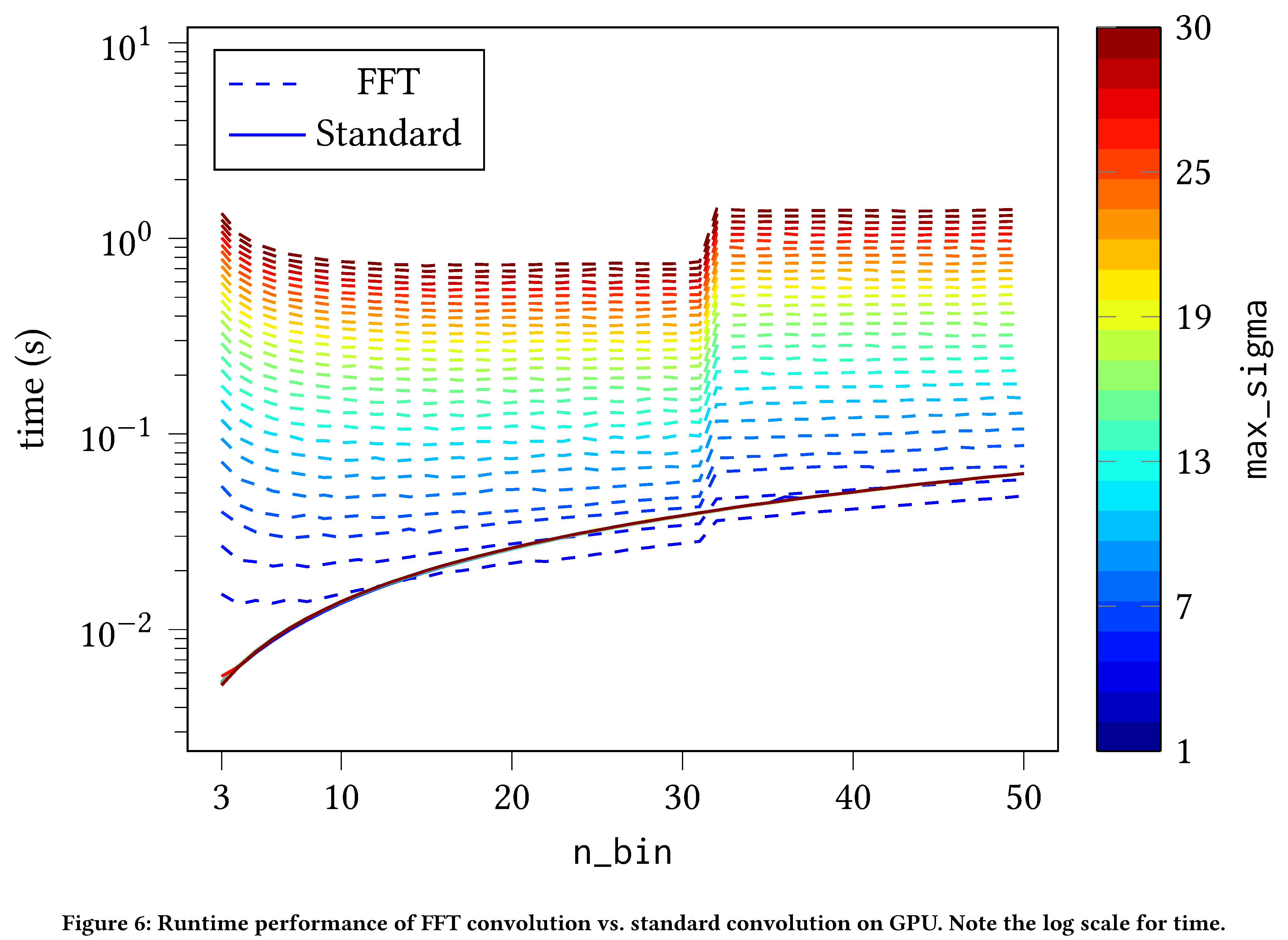
max_sigma (i.e. the widths of the Gaussian filters). On the other
hand, CPU as compared with our bespoke FFT convolution implementation is
even more encouraging; FFT convolutions make the GPU implementation even
faster. They are weakly dependent (approximately log-linear) on n_bin
but constant with respect to max_sigma (see
Figure 8).
In fact, we see that for $\mathtt{max_sigma} > 2$ and
$\mathtt{n_bin} > 10$ it already makes sense to use FFT convolution
instead of the standard PyTorch convolution.
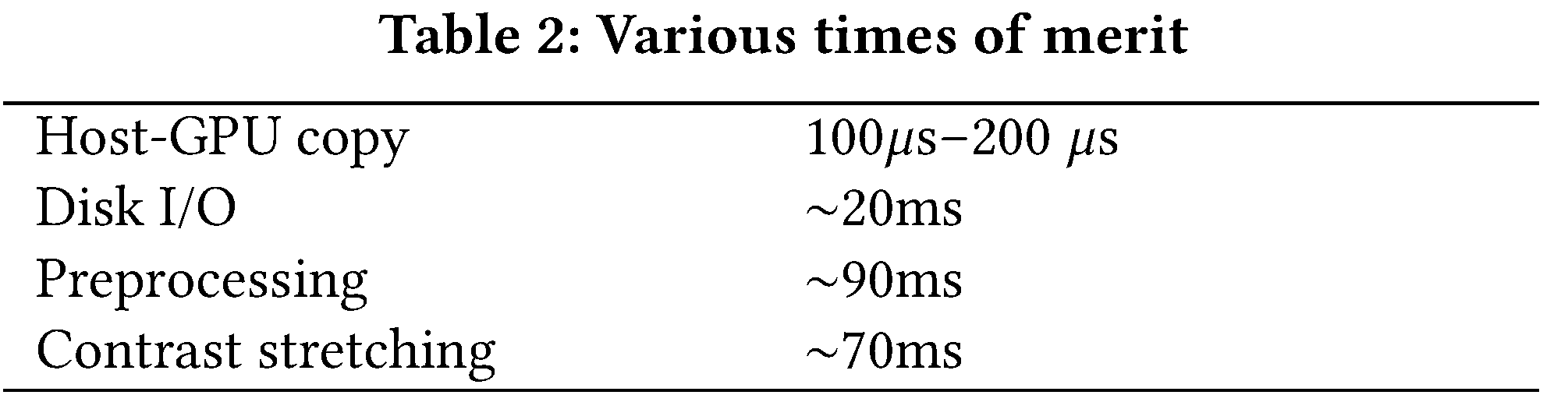
Some discussion of I/O and Host-GPU and GPU-Host copy is warranted (see
Table 6).
Our measurements show that for $1000 \times 1000$ grayscale images,
Host-GPU copy times range from 100$\mu$s–200 $\mu$s, depending on
whether or not we copy from page-locked memory (by setting
pin_memory=True in various places). This Host-GPU transfer is strongly
dominated by disk I/O and initial preprocessing, which is common to both
CPU and GPU implementations. The bulk of the preprocessing time is
consumed by the contrast stretching operation, whose purpose is to
approximately fix the threshold at which we reject spurious maxima in
scale-space. We further note that since most of our samples have
${\sim}1000$ blobs, GPU-Host copy time (i.e. ${\sim}1000$ tuples of
$(x,y,\sigma)$) is nominal. Therefore Host-GPU and GPU-Host copy times
are not onerous and do not dilute the performance improvements of our
GPU implementation.
We have deployed our GPU implementation of DoG as an on-demand analysis tool through the MDML platform. The MDML uses funcX [15] to serve the DoG tool on a HPC GPU-enhanced cluster at Argonne National Laboratory. The GPU cluster shares a high performance network with the FSP instrument (284$\mu$s average latency). Our DoG implementation requires 100ms on average to analyze a PLIF image. This processing rate is sufficient to provide online analysis of PLIF data as they are generated, enabling near real-time feedback and optimization of configurations.
Related work
There is much historical work in this area employing classical methods and some more recent work employing neural network methods. A useful survey is Ilonen et al. [16]. Yuen et al. [17] compare various implementations of the Hough Transform for circle finding in metallurgical applications. Strokina et al. [18] detect bubbles for the purpose of measuring gas volume in pulp suspensions, formulating the problem as the detection of concentric circular arrangements by using Random Sample and Consensus (RANSAC) on edges. Poletaev et al. [19] train a CNN to perform object detection for studying two-phase bubble flows. The primary impediment to applying Poletaev’s techniques to our problem is our complete lack of ground-truthed samples, which prevents us from being able to actually train any learning machine, let alone a sample-inefficient machine such as a CNN [20]. All of these methods, amongst other drawbacks, fail to be performant enough for real-time use. For example, Poletaev’s CNN takes ${\sim}$8 seconds to achieve 94%–96% accuracy. One method that merits further investigation is direct estimation of the volume distribution from the power spectrum of the image [21].
As pertaining to real-time optimization and steering, Laszewski et al. [22] and Bicer et al. [23] demonstrate real-time processing and consequent steering of synchrotron light sources. Steering using other compute node types such as FPGAs has also been studied [24]. Vogelgesang et al. [25] used FPGAs in concert with GPUs in streaming mode to analyze synchrotron data. The key difference between Vogelgesang’s and our work is we do not need to use direct memory access to achieve low-latency results.
Conclusion
We have presented a method for the inference of droplet size distribution in PLIF images of FSP. We briefly introduced the scale-space representation of an image and discussed several detectors that operate on such a representation. Identifying the DoG operator as striking the right balance between accuracy and performance, we implemented it on GPU. We then compared our GPU implementation (and a refinement thereof) against a reference implementation. Our comparison demonstrates an order of magnitude improvement over the reference implementation with almost no decrease in accuracy. These improvements make it possible to perform online analysis of PLIF images using a GPU-enhanced cluster, enabling online feedback and optimization of the FSP instrument. Future work will focus on improving memory access times and disk I/O optimizations.