• Introduction
  • Definitions
    • Channel model
    • Strings and things
    • Codes
    • Entropy
• Lemmas
  • Shannon Entropy
  • Gibbs’ inequality
  • Kraft-McMillan Inequality
• Shannon source coding theorem for symbol codes
• Proofs
  • Shannon entropy
  • Gibbs’ inequality
  • Kraft–McMillan inequality
• Footnotes

Introduction

Shannon’s source coding theorem accomplishes two things:

1. Sets absolute bounds on data compression.
2. Operationally¹ defines Shannon entropy.

By “sets absolute bounds on data compression” we mean that it is asymptotically² almost never³ possible to compress a sequence of symbols such that the bit rate⁴ is less than the Shannon entropy of the source, without almost surely⁵ losing information. Note, that, a priori, the bit rate depends on the encoding scheme, but indeed the source coding theorem precisely shows that there is a lower bound on this bit rate irrespective of the encoding. On the other hand, it is possible to get arbitrarily close to the optimal bit rate (namely the Shannon entropy of the source).

The rest of this article proceeds as follows: basic definitions, necessary lemmas (proofs relegated to the Proofs), statement and proof of the source coding theorem. We roughly follow and recapitulate the proofs in Shannon’s original 1948 article A Mathematical Theory of Communication and various relevant wikipedia articles.

A few words on syntax: bolding is used to indicate in situ definitions rather than emphasis, italics are used for emphasis, \(:=\) is used for defining/declaring mathematical objects, footnotes are used (liberally) for colloquial terms that might be unknown to some readers and various tidbits, “double quotes” are used to indicate informal use of the quoted word or phrase.

Definitions

Channel model

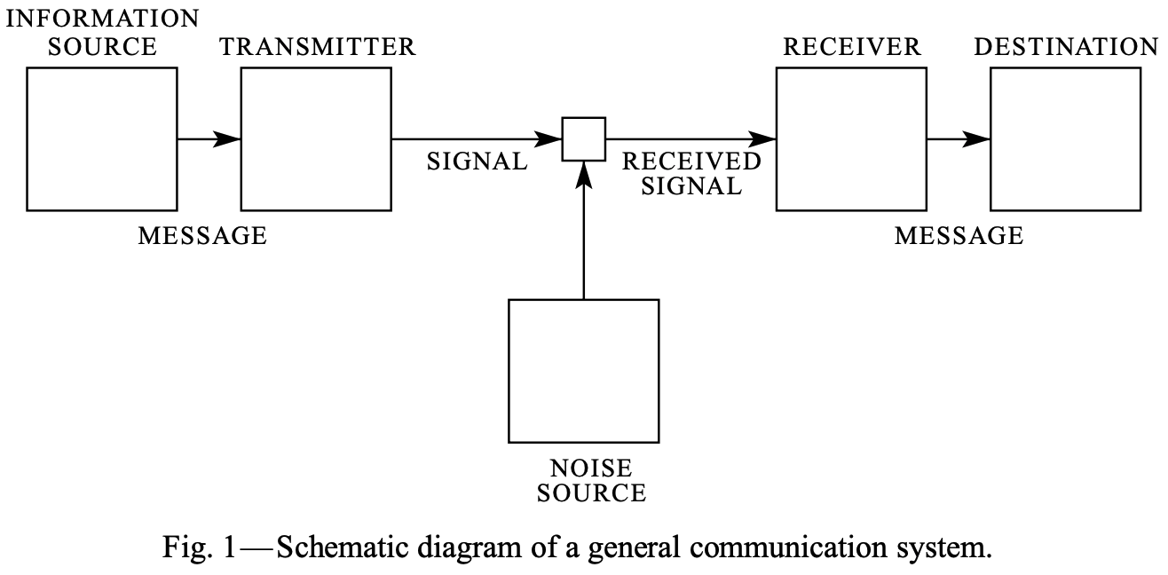
The above is from Shannon’s original paper. An information source is that which produces a message or sequence of messages; a message can be anything from binary digits \(\{0,1\}\) to a television broadcast. A transmitter operates on the messages (potentially transforming or encoding them) in order to produce a signal suitable for transmission over a medium (called the channel). The transformation performed by the transmitter should be invertible such that the receiver may invert it and pass it along to the interested party at the destination. While we do not here consider noisy channels, the noise source is a model for perturbation of the transmitted signal due to various phenomena (e.g. decay to due impurities in the medium or packet loss).

Strings and things

A string \(s\) is a finite sequence of elements, called symbols, of a fixed set, called an alphabet \(\Sigma\). For example, \(s = 123\) with \(\Sigma = \{0, 1, \dots, 9\}\). Note, by convention the empty string \(\epsilon\) is a member/symbol of every alphabet. The set of all strings of length \(n\) (for some fixed \(n\)) is denoted \(\Sigma^n\). The set of all finite length strings over the alphabet \(\Sigma^*\), where \(*\) is the Kleene closure of \(\Sigma\), is defined as

\[\Sigma^* := \bigcup _{i \in \mathbb {N} }\Sigma ^{i}\]

The set of all infinite length strings is denoted \(\Sigma^\omega\). The set of all strings is defined as \(\Sigma^\infty := \Sigma^* \cup \Sigma^\omega\).

Codes

A code \(C\) is a total⁶ mapping between a source alphabet \(\Sigma_1\) and the Kleene closure \(\Sigma_2^*\) of another alphabet \(\Sigma_2\), called the target or destination alphabet. That is to say \(C : \Sigma_1 \rightarrow \Sigma_2^*\). Strings in \(\Sigma_2^*\) are called codewords. For example, with \(\Sigma_1 := \{ a,b,c\}\) and \(\Sigma_2 := \{ 0, 1\}\)

\[C' := \{\, a\mapsto 0, b\mapsto 01, c\mapsto 011\,\}\]

is a code. Note that a code \(C\) naturally extends to \(C^* : \Sigma_1^* \rightarrow \Sigma_2^*\) by concatenation. We say that \(C\) encodes \(\Sigma_1\) and that any string of target symbols such that \(C^*(s) \in \Sigma_2^*\) is an encoding of a string of source symbols in \(s \in \Sigma_1^*\). \(C\) is called a variable-length code if the length of the codewords assigned to \(s \in \Sigma_1\) varies. Alternatively

\[C'' := \{\, a\mapsto 001, b\mapsto 010, c\mapsto 011\,\}\]

is a fixed-length code (wrt the same alphabets) because the number of symbols used is constant (three). The code \(C'\) is also uniquely decodable: any string of target symbols (bit strings) cannot end in a 0 (and therefore we can partition any concatenated encoding on 0 to recover the constituent codewords). On the other hand, \(C'\) is not a prefix-free code (also annoyingly called a prefix code) because \(a\) is a prefix of \(b\) (written \(a\sqsubseteq b\)). An example of a prefix-free code is

\[C''' := \{\, a\mapsto 0, b\mapsto 10, c\mapsto 110\,\}\]

A prefix-free code is uniquely decodable but the converse isn’t necessarily true (notice that \(C'''\) is the reversal of \(C'\)).

Entropy

Suppose we have a discrete⁷ information source; is there a plausible measure of how much “information” is produced and at what rate? Firstly, what is an appropriate formal model for information? Consider that, in general, messages received by the destination that are highly correlated, or, alternatively, about which the destination is quite certain are “uninformative”. For example, letters in a word appear in an order according to spelling conventions of a language and therefore (assuming the receiver is a fair speller) much of the word is unnecessarily transmitted. An immediate implication is that sources that produce “surprising” messages or, alternatively, messages that the destination is “uncertain” about, are highly informative. Furthermore, we conclude that the model of information should entail probability distributions (in order to measure uncertainty) over outcomes (messages).

Thus, suppose we have a collection of possible outcomes \(A_i\) with corresponding probabilities of occurring \(p_i\) and that these probabilities are all that is known about the outcomes. What properties should a measure \(H\) of information have?

1. \(H\) should be a continuous function of only the \(p_i\).
2. If \(p_i = 1/n\), then \(H(p_1, p_2, \dots, p_n) = H(n)\); with equally likely outcomes, increasing the quantity of outcomes increases the uncertainty at the destination.

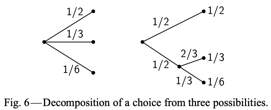
3. If an outcome has structure in and of itself, i.e. is actually the result of a sequence of decisions, \(H\) should incorporate that structure as a weighted average of constituent \(H_j\); consider the following decision tree representation of a probability distribution

   

   The above suggests that

   \[H \left(\frac{1}{2}, \frac{1}{3}, \frac{1}{6}\right) = H_a \left(\frac{1}{2}, \frac{1}{2}\right) + \frac{1}{2} H_b \left(\frac{2}{3}, \frac{1}{3}\right)\]

   where \(H_a \left(\frac{1}{2}, \frac{1}{2}\right)\) corresponds to the uncertainty associated with the first decision (at the root) and \(H_b \left(\frac{2}{3}, \frac{1}{3}\right)\) corresponds to the conditional subsequent uncertainty (and where the \(\frac{1}{2}\) coefficient captures the uncertainty associated with conditionality). Note that there’s a trivial term omitted \(\frac{1}{2} H \left( \frac{1}{2} \right)\) because \(H \left( \frac{1}{2} \right) = 0\) (since there’s no uncertainty associated with a single “choice”). In general \(H\) should have the property that

   \[H = \sum_j P_j H_j\]

   for subsequences of information measures \(H_j\), each with conditional probability \(P_j\).

Lemmas

Shannon Entropy

The three desired properties for a measure of information uniquely constrain \(H\) to be defined

\[H := -K \sum_{i=1}^n p_i \log p_i\]

where \(K\) is tantamount to specifying units for the measure. With \(K := 1\), \(H\) becomes Shannon entropy of a discrete probability distribution. Note that \(H\) can be rewritten as

\[H = -K \sum_{i=1}^n p_i \log p_i = K \sum_{i=1}^n p_i \log \left( \frac{1}{p_i}\right)\]

The \(\log \left( \frac{1}{p_i}\right)\) terms in the sum more obviously illustrate that \(H\) measures uncertainty; intuitively uncertainty about an outcome is inversely proportional to the probability of that event occurring.

Gibbs’ inequality

Gibbs’ inequality is a statement about the relationship of the Shannon entropy of a discrete probability distribution to its cross entropy with any other discrete probability distribution.

Theorem: Let \(P=\{p_{1},\dots ,p_{N}\}\) and \(Q=\{q_{1},\dots ,q_{n}\}\) be two discrete probability distributions (on \(\{1, \dots, N\}\)). Then

\[\begin{aligned} H(P) \leq H(P, Q) \end{aligned}\]

where \(H(P) := -\sum_{i=1}^{N}p_{i}\log p_{i}\) and \(H(P,Q) := -\sum_{i=1}^{N}p_{i}\log q_{i}\), with equality iff \(p_{i}=q_{i}\).

Kraft-McMillan Inequality

Kraft-McMillan gives a necessary and sufficient condition for the existence of a uniquely decodable (or prefix) code for a given set of codeword lengths.

Theorem: Let \(\Sigma_1 := \{ s_1, \dots, s_N \}\) be a source alphabet to be encoded into uniquely decodable code over an alphabet \(\Sigma_2\) of size \(\left| \Sigma_2 \right| = r\) with codeword lengths \(\{\ell_1, \dots, \ell_N \}\). Then

\[\sum_{i=1}^N r^{-\ell_i} \leq 1\]

Conversely, if \(\{\ell_1, \dots, \ell_N \,\mid\, \ell_i \in \mathbb{N} \}\) satisfy the above inequality, then there exists a uniquely decodable (or prefix) code over an alphabet of size \(r\) with corresponding codeword lengths.

Shannon source coding theorem for symbol codes

Let \(\Sigma_1, \Sigma_2\) be two finite alphabets and \(X\) a random variable with \(X \in \Sigma_1\). Suppose \(C : \Sigma_1 \rightarrow \Sigma_2^*\) is any uniquely decodable code that has minimal expected encoding length, i.e. for \(L(X) := \left| C(X) \right|\), the length of the encoding of \(X\), the encoding \(C\) has the property that \(\mathbb{E}_C[L] \leq \mathbb{E}_{C'}[L']\) for any other uniquely decodable \(C'\) (where \(L' := \left| C'(X) \right|\)). Then

\[\frac{H(X)}{\log _{2} \left| \Sigma_2 \right|}\leq \mathbb {E}_C [L]<\frac {H(X)}{\log _{2} \left| \Sigma_2 \right|}+1\]

where \(\lvert \Sigma_2 \rvert\) is the cardinality of \(\Sigma_2\). This means that the lower bound on encoding length (on average) is \(\frac{H(X)}{ \log_2 \left| \Sigma_2 \right| }\). The question remains whether there exist codes that achieve this lower bound; though we don’t prove it here, Huffman codes do attain the lower bound.

We now prove the source coding theorem for symbol codes (rather than in full generality).

Proof: Let \(X\) be a random variable with draws \(x_i \in \Sigma_1\) for \(i = 1, \dots, N\), drawn according to probabilities \(p_i\) and let \(\ell_i := L(C(x_i))\) for some encoding \(C\). Define \(a := \left| \Sigma_2 \right|\) (cardinality) and \(q_i = \frac{a^{-\ell_i}}{R}\) for \(i = 1, \dots, N\), with \(R := \sum_{i=1}^N a^{-\ell_i}\) (i.e. such that \(\sum_{i=1}^N q_i = 1\) and the \(q_i\) comprise a discrete probability distribution). Then

\[\begin{aligned} H(X) &= - \sum_{i=1}^N p_i \log p_i \\ &\leq - \sum_{i=1}^N p_i \log q_i \quad \mbox{by Gibb's inequality} \\ &= - \sum_{i=1}^N p_i \log a^{\ell_i} + \sum_{i=1}^N p_i \log R \\ &= - \sum_{i=1}^N p_i \log a^{\ell_i} + \log R \quad \mbox{by } \sum_i p_i = 1\\ &\leq - \sum_{i=1}^N -\ell_i p_i \log a \quad \mbox{by Kraft-McMillian inequality } \implies \log R \leq 0 \\ &\leq \mathbb{E}_C \left[ L\cdot \log a \right] \\ &= \mathbb{E}_C \left[ L \right] \cdot \log \left| \Sigma \right| \end{aligned}\]

This then gives the lower bound on \(\mathbb{E}_C \left[ L \right]\). For the upper bound we set \(\ell_i := \lceil -\log_a p_i \rceil\) so that

\[-\log _{a}p_{i}\leq \ell_{i}<-\log _{a}p_{i}+1\]

and hence

\[a^{-\ell_{i}}\leq p_{i} \implies \sum_{i=1}^N a^{-\ell_{i}} \leq 1\]

By Kraft’s inequality there exists a prefix code having such words lengths \(\ell_i\) and thus

\[\begin{aligned} \mathbb{E}_C \left[ L \right] &= \sum_{i=1}^N p_i \ell_i \\ &< \sum_{i=1}^N p_i \left( -\log_a p_i + 1 \right) \\ &= \left( \sum_{i=1}^N -p_i \frac{\log p_i}{\log a} \right) + 1 \quad \mbox{by } \sum_i p_i = 1\\ &= \frac{H(X)}{\log a} + 1 \\ &= \frac{H(X)}{ \log \left| \Sigma \right|} + 1 \\ \end{aligned}\]

Proofs

Shannon entropy

Starting with the simplest case; let \(H(n) := H \left( \frac{1}{n}, \frac{1}{n}, \dots, \frac{1}{n} \right)\) for arbitrary finite \(n\). Consider \(n = j\cdot k\) i.e. group \(n\) outcomes into \(j\) groups of \(k\) equiprobable outcomes. From the decomposition property (property 3) we have

\[\begin{aligned} H(n) &= H(jk) \\ &= H(j) + \sum_{i=1}^j \left(\frac{1}{j}\right) H(k) \\ &= j \left(\frac{1}{j}\right) H(k) \\ &= H(j) + H(k) \end{aligned}\]

Thus, by the equivalence (exponentiation \(\iff\) iterated multiplication), we have \(H(s^m) = m H(s)\) and \(H(t^n) = n H(t)\) for arbitrary \(t, s, n, m \in \mathbb{N}\). In particular, we can choose \(m,n\) to satisfy

\[\begin{aligned} s^m \leq t^n < s^{m+1} &\iff m \log s \leq n \log t < (m+1) \log s \quad \mbox{by monotonicity of log} \\ &\iff \frac{m}{n} \leq \frac{\log t}{\log s} < \frac{m}{n} + \frac{1}{n} \\ &\iff \left|\frac{m}{n} - \frac{\log t}{\log s} \right| < \frac{1}{n} \end{aligned}\]

Similarly (using the monotonicity of \(H\))

\[\begin{aligned} H(s^m) \leq H(t^n) < H(s^{m+1}) &\iff mH(s) \leq nH(t) < (m+1)H(s) \\ &\iff \left|\frac{m}{n} - \frac{H(t)}{H(s)} \right| < \frac{1}{n} \end{aligned}\]

Then by the triangle inequality

\[\left| \frac{H(t)}{H(s)} - \frac{\log t}{\log s} \right| \leq \left|\frac{m}{n} - \frac{\log t}{\log s} \right| + \left|\frac{m}{n} - \frac{H(t)}{H(s)} \right| < \varepsilon = \frac{2}{n}\]

and hence \(H(t) = K \log t\).

Now suppose we have \(N\) possible outcomes with \(p_i \in \mathbb{Q}\). Finding a common denominator we can write

\[p_i = \frac{n_i}{\sum_{j=1}^N n_j} = n_i \cdot \left(\frac{1}{\sum_{j=1}^N n_j}\right)\]

i.e. each \(p_i\) can be partitioned into \(n_i\) equiprobable outcomes. Looking at it another way, we can consider the entropy for the total number of outcomes \(\sum_{i=1}^N n_i\) as a composite entropy, based on a decision on \(i\) with probability \(p_i\) and then the weighted average of the entropies of \(n_i\) equiprobable choices. Therefore, by the third property again

\[K \log \sum_{i=1}^N n_i = H \left( \sum_{i=1}^N n_i\right) = H \left(p_1, \dots, p_n \right) + \sum_{i=1}^N p_i H\left(n_i\right)\]

Hence (by \(\sum_{i=1}^N p_i = 1\))

\[\begin{aligned} H \left(p_1, \dots, p_n \right) &= K \left( \left( \sum_{i=1}^N p_i \right) \log \sum_{i=1}^N n_i -\sum_{i=1}^N p_i \log n_i \right) \\ &= K \left( \left( \sum_{i=1}^N p_i \log \sum_{j=1}^N n_j \right) -\sum_{i=1}^N p_i \log n_i \right) \\ &= K \left( \sum_{i=1}^N p_i \log \frac{\sum_{j=1}^N n_j }{n_i} \right) \\ &= -K \sum_{i=1}^N p_i \log p_i \end{aligned}\]

By continuity we can extend this to all of \(\mathbb{R}\). Setting \(K\), as already mentioned, sets the units of \(H\) and is a matter of convention; choosing \(K = 1 \log 2\) sets the units as bits, while choosing \(K = 1\) sets the units as nats.

Gibbs’ inequality

Proof: Let \(I := \{i \, \mid \, p_i > 0 \}\). Then by \(\log x \leq x - 1\) for \(x > 0\) and \(\log x = x - 1\) for \(x = 1\) we have

\[\begin{aligned} \sum_{i \in I} p_i \log \frac{q_i}{p_i} &\geq -\sum_{i \in I} p_i \left( \frac{q_i}{p_i} - 1\right)\\ &= -\sum_{i \in I} q_i + \sum_{i \in I} p_i \\ &= -\sum_{i \in I} q_i + 1 \quad \mbox{since } \sum_{i \in I}^N p_i = 1 \\ &\geq 0 \qquad\qquad\qquad \mbox{since } \sum_{i \in I}^N q_i \leq 1 \end{aligned}\]

Thus, over the index set \(I\) we have

\[-\sum _{i\in I}p_{i}\log p_{i} \leq -\sum _{i\in I}p_{i}\log q_{i}\]

We can extend this to all of \(\{1, \dots, N\}\) by noting that \(\lim_{p \rightarrow 0} p \log p = 0\) and \(\lim_{q \rightarrow 0} -\log q = \infty\).

Equality holds iff

\[\sum_{i} p_i \log \frac{q_i}{p_i} = 0\]

which holds iff \(\frac{q_i}{p_i} = 1\).

Interesting note: the degree to which equality fails, i.e. \(H(P) - H(P, Q)\), is called the Kullback–Leibler divergence or relative entropy

\[D_{\mathrm {KL} }(P\mid Q)= \sum _{i=1}^{n}p_{i}\log {\frac {p_{i}}{q_{i}}}\geq 0\]

Kraft–McMillan inequality

We first prove both directions for prefix codes and then prove only the forward direction for uniquely decodable codes (omitting the converse because the converse wrt prefix codes implies the converse for uniquely decodable codes)⁸.

Proof for prefix codes: Suppose \(\ell _{1}\leq \ell _{2}\leq \cdots \leq \ell _{N}\) and let \(A\) be the full⁹ \(r\)-ary tree of depth \(\ell_N\). Every word of length \(\ell \leq \ell_N\) corresponds to a node in this tree; just descend the tree, at each depth choosing the child, of \(r\) children, corresponding to the symbol at the position in the word corresponding to the depth. Therefore, for such a prefix code, the \(i\)th codeword, having length \(\ell_i\) corresponds to some node \(v_i \in A\) at depth \(\ell_i\). Let \(A_i\) be the set of all leaf nodes of the subtree rooted at \(v_i\). Note that the subtree, having \(v_i\) as the root, is of height \(\ell_N - \ell_i\) and hence

\[\left| A_i \right| = r^{\ell_N - \ell_i}\]

Since the code is a prefix code, the \(i\)th and \(j\)th codewords have disjoint subtrees in \(A\) and therefore

\[A_i \cap A_j = \emptyset \quad \mbox{for } i \neq j\]

Thus, since the total number of nodes at depth \(\ell_N\) is \(r^{\ell_N}\)

\[\left|\bigcup _{i=1}^{N}A_{i}\right|=\sum _{i=1}^{N}|A_{i}|=\sum _{i=1}^{N}r^{\ell _{N}-\ell _{i}}\leq r^{\ell _{N}}\]

and dividing the last inequality by \(r^{\ell _{N}}\) completes the proof of the forward direction.

Conversely, assume \(\{\ell_1, \dots, \ell_N \,\mid\, \ell_i \in \mathbb{N} \}\) satisfy the above inequality. Then we build a suitable prefix code by consulting the same \(r\)-ary tree \(A\). We proceed inductively: for \(\ell_1\) pick any node that is a child of the root and remove the subtree rooted at it in order to prevent any forthcoming codewords from containing it as a prefix. This eliminates \(r^{\ell_N - \ell_1}\) leaf nodes from \(A\). Repeat for \(\ell_2, \dots, \ell_N\). In toto this eliminates

\[\sum _{i=1}^{N}r^{\ell _{n}-\ell _{i}} \leq r^{\ell_N}\]

leaf nodes. By Kraft’s inequality (multiplying both sides by \(r^{\ell_N}\)) there are enough nodes in \(A\) to complete the process.

Forward proof for uniquely decodable codes:

Let \(C\) be a uniquely decodable code and \(C^K\) be its extension from symbols in \(\Sigma_1\) to \(K\)-length sequences of symbols \(s_1, s_2, \dots, s_K\) by concatenation (producing codewords that are the concatenations of individual codewords in \(C\)). Note that

\[L(C^K(s_1, s_2, \dots, s_K)) = \sum_{i=1}^K L(C(s_i))\]

Consider the quantity

\[\begin{aligned} \left( \sum_{s \in \Sigma_1} r^{-L(C(s))} \right)^K &= \underbrace{\left( \sum_{s \in \Sigma_1} r^{-L(C(s))} \right) \left( \sum_{s \in \Sigma_1} r^{-L(C(s))} \right) \cdots \left( \sum_{s \in \Sigma_1} r^{-L(C(s))} \right)}_{K \text{ independent sums}} \\ &= \sum_{s_1 \in \Sigma_1} \sum_{s_2 \in \Sigma_1} \cdots \sum_{s_K \in \Sigma_1} r^{-\sum_{i=1}^K L(C(s_i))} \\ &= \sum_{s_1, s_2, \dots, s_K} r^{-L(C^K(s_1, s_2, \dots, s_K))} \end{aligned}\]

In the last line the sum runs over all possible \(K\)-length sequences of symbols.

Note that \(C^\ell\) is uniquely decodable for all \(\ell\) (including \(\ell = K\)). Therefore, if \(n_\ell\) is the number of sequences whose concatenated codewords have length \(\ell\) and \(r^\ell\) is the total possible number of codewords of length \(\ell\) then \(n_\ell \leq r^\ell\) (because if \(n_\ell > r^\ell\) then by the pigeonhole principle two sequences would map to the same codeword, thereby contradicting unique decodability). Then we can rewrite the sum above as running over lengths of concatenated codewords (from \(K \cdot \ell_1\) to \(K \cdot \ell_{N}\)) rather than running explicitly over the sequences of symbols themselves:

\[\begin{aligned} \sum_{s_1, s_2, \dots, s_K} r^{-L(C^K(s_1, s_2, \dots, s_K))} &= \sum_{\ell = K \cdot \ell_1}^{K \cdot \ell_{N}} n_\ell r^{-\ell} \\ &\leq \sum_{\ell = K \cdot \ell_1}^{K \cdot \ell_{N}} r^\ell r^{-\ell} \\ &= K (\ell_N - \ell_1 + 1) \end{aligned}\]

Finally we arrive at

\[\left( \sum_{s \in \Sigma_1} r^{-L(C(s))} \right)^K \leq K (\ell_N - \ell_1 + 1)\]

or

\[\sum_{s \in \Sigma_1} r^{-L(C(s))} \leq \left( K (\ell_N - \ell_1 + 1) \right)^{1/K}\]

or

\[\sum_{i=1}^N r^{-\ell_i} \leq \left( K (\ell_N - \ell_1 + 1) \right)^{1/K}\]

and since the left-hand side is independent of \(K\), taking the limit of the right-hand side as \(K \rightarrow \infty\) produces the desired upper bound.

Footnotes