• A slew of definitions about graphs
• Representations of graphs
• Breadth-first search
• Dijkstra’s Shortest Path (Optional)
• Depth-first search
• Tangent: parentheses
• Topological Sort
• Strongly Connected Components
• Footnotes

A slew of definitions about graphs

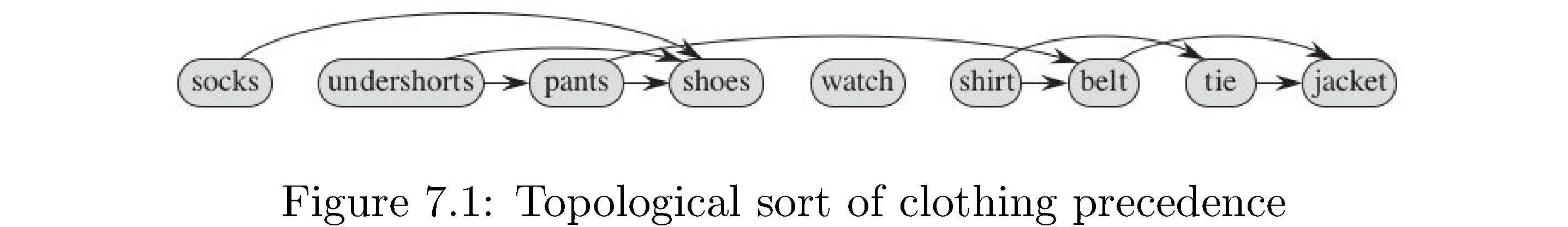
A graph \(G\) is a pair \(\left(V,E\right)\) of things: a set \(V\) of vertices and a set \(E\) of edges. Vertices are an abstraction: they can represent anything from cities, people, jobs, classes, etc. to other vertices. The edges give relational information: if two vertices \(u,v\) are related then there will be an edge saying as much, usually written \(\left(u,v\right)\), in the set of edges. If the relational information is symmetric¹ - \(u\) related to \(v\) is the same as \(v\) related to \(u\) - then the edges are undirected and the the graph is an undirected graph. If the relational information isn’t symmetric² - \(u\) related to \(v\) isn’t the same as \(v\) related to \(u\) - then the edges are ordered pairs, meaning \(\left(u,v\right)\neq\left(v,u\right)\) (just like the \(xy\) plane ordered pairs \(\left(1,2\right),\left(2,1\right)\) aren’t equal), are called directed edges or arrows, and the graph is a directed graph. Figure 1 is a directed graph. The vertices are clothes you would put on when getting dressed and the edges (arrows) represent precedence (you have to put on your underwear before your pants and your pants before your belt).

In an undirected graph the jargon is that the edge \(\left(u,v\right)\) is incident on the vertices \(u\) and \(v\). In a directed graph we need to convey information about the direction of the edge so we say that edge \(\left(u,v\right)\) is incident from \(u\) and incident to \(v\). I’ve never heard anyone say this but it is true that it’s important to convey direction for all edges when describing edges in an undirected graph. If two vertices have an edge connecting them then they’re adjacent.

A subraph \(G'=\left(V',E'\right)\) of a graph \(G\) is any \(E'\subset E\) and \(V'\subset V\). Given some \(V'\subset V\) the subgraph induced on \(G\) by \(V'\) is the graph \(G'=\left(V',E'\right)\) where \(E'\) is the set of edges in \(E\) connecting vertices in \(V'\), i.e. \(E'=\left\{ \left(u,v\right)\in E\big|u,v\in V'\right\}\). It’s basically the graph you get by throwing away some vertices.

In a graph the degree of a vertex is the number of edges incident on it (i.e. just the number of edges connected to it). In a directed graph we need to also distinguish between edges into the vertex and edges leaving (but just the degree is still the total number): the in-degree of a vertex is number of edges coming into the vertex and the out-degree ** is the number of edges leaving the vertex. An **isolated vertex is one whose degree is 0 (like ‘watch‘ in figure 1).

A path of length \(k\) from vertex \(v_{0}\) to \(v_{k}\) is a sequence of vertices \(\left(\underbrace{v_{0},v_{1},\dots,v_{k}}_{k+1}\right)\) (i.e. a walk along the edges from \(v_{0}\) to \(v_{k}\)). The “\(k\) length” comes from the \(k\) edges connecting vertices not the \(k+1\) vertices: \(\left\{ \underbrace{\left(v_{0},v_{1}\right)}_{\text{1st}},\underbrace{\left(v_{1},v_{2}\right)}_{\text{2nd}},\dots,\underbrace{\left(v_{k-1},v_{k}\right)}_{k\text{th}}\right\}\). Note also that there’s no requirement that the edges or vertices be distinct, meaning a path that retraces its steps is fine. A simple path is one where all the vertices in \(\left(v_{0},v_{1},\dots,v_{k}\right)\) are distinct, i.e. that doesn’t retrace its steps. A cycle is a path where \(v_{0}=v_{k}\), i.e. ends up where it starts. A simple cycle is a cycle that doesn’t retrace its steps. A graph with no cycles is called acyclic.

A graph is connected if there’s a path from any vertex to any other vertex. A graph that isn’t connected isn’t “disconnected”! It’s just not connected. The graph in figure 1 is not connected because there’s no path from any vertex to ‘watch‘. Note in a directed graph you can’t “go backwards” along edges so also there’s no path from ‘pants‘ to ‘undershorts‘. A connected component \(V'\subset V\) of an undirected graph is a set of vertices such that the graph \(G'\) induced on \(G\) by \(V'\) is connected, i.e. it’s a subset of the original vertices where any vertex in that subset is reachable from any other in that subset. In figure 1 if you flip the edge \(\left(\text{undershorts},\text{shoes}\right)\) to \(\left(\text{shoes},\text{undershorts}\right)\) then \(V'=\left\{ \text{undershorts},\text{shorts},\text{shoes}\right\}\) becomes a connected component because you can just “go around the path” from any of them to any other. There can be several connected components in a graph. In figure 1 if you also flip the edges \(\left(\text{shirt},\text{tie}\right)\) and \(\left(\text{tie},\text{jacket}\right)\) then \(V'=\left\{ \text{undershorts},\text{pants},\text{shoes}\right\}\) and \(V''=\left\{ \text{shirt},\text{tie},\text{jacket}\right\}\) become connected components (but are not connected to each other).

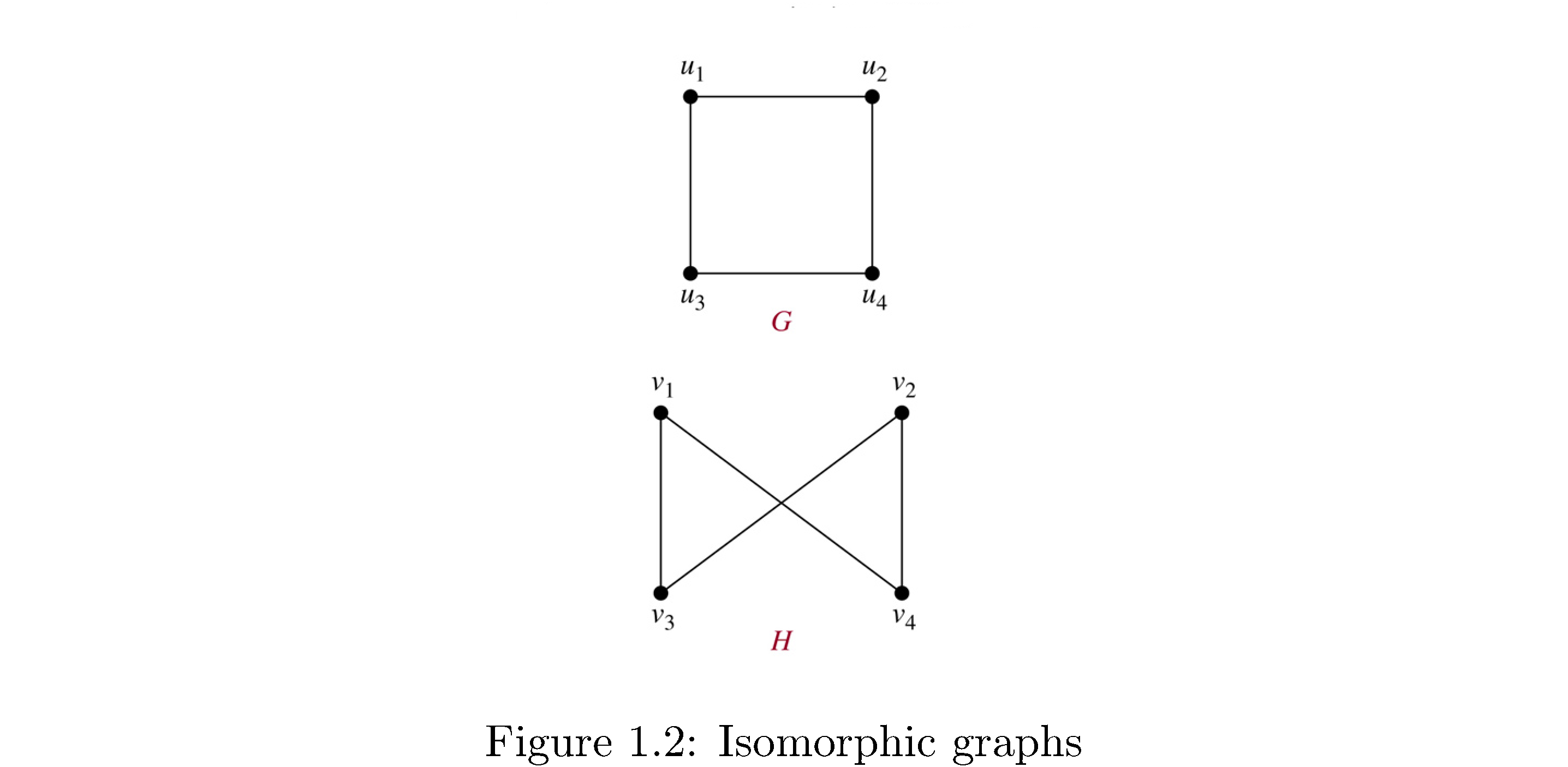
Two graphs \(G,G'\) are isomorphic if there’s a bijection \(f:V\rightarrow V'\) such that \(\left(u,v\right)\in E\iff\left(f\left(u\right),f\left(v\right)\right)\in E'\), i.e. essentially the same except for a relableing of the vertex names. Figure 2 shows two isomorphic graphs because the mapping

\[\begin{align} f\left(u_{1}\right) &= v_{1}\\ f\left(u_{2}\right) &= v_{4}\\ f\left(u_{3}\right) &= v_{3}\\ f\left(u_{4}\right) &= v_{2}\end{align}\]

works (all you do is “twist” vertices \(u_{2},u_{4}\)).

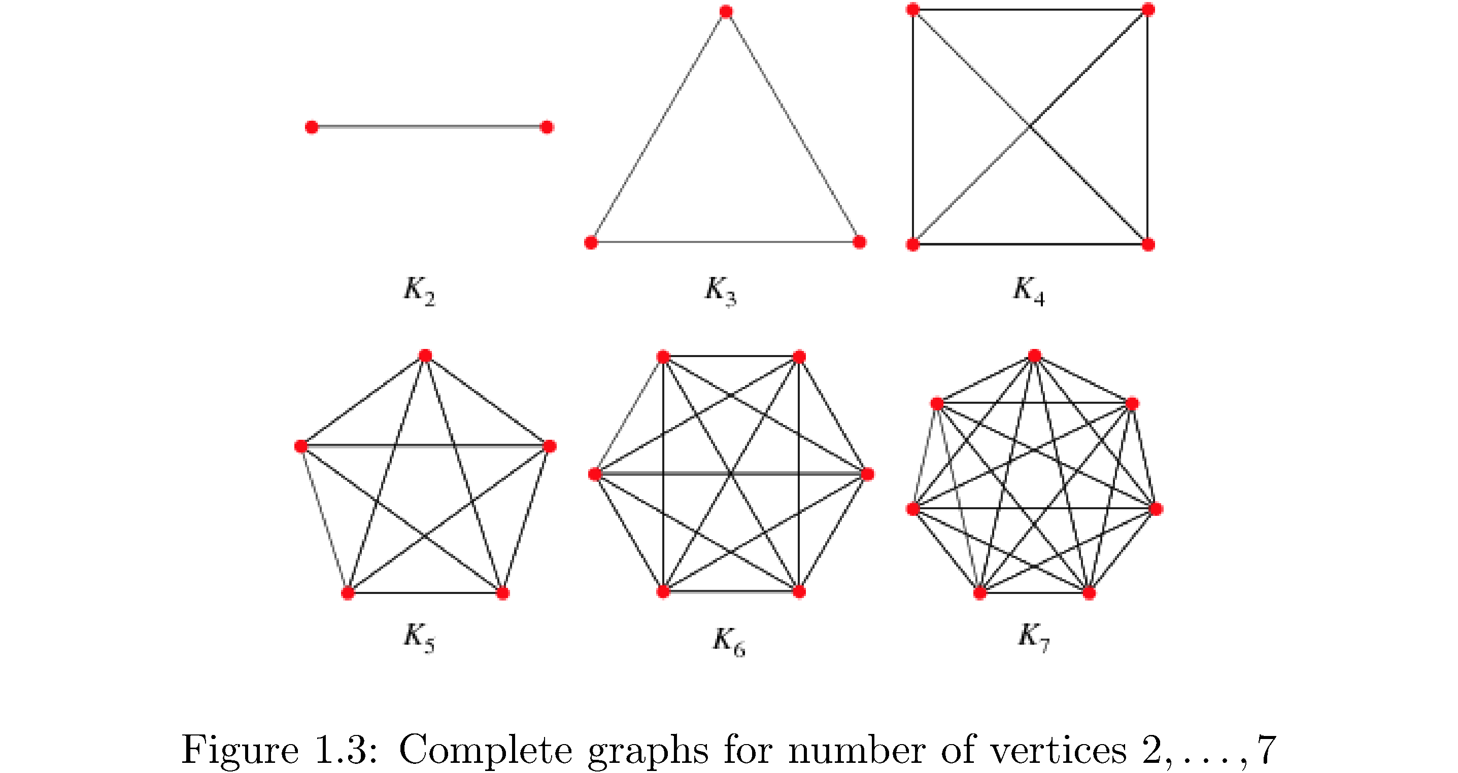
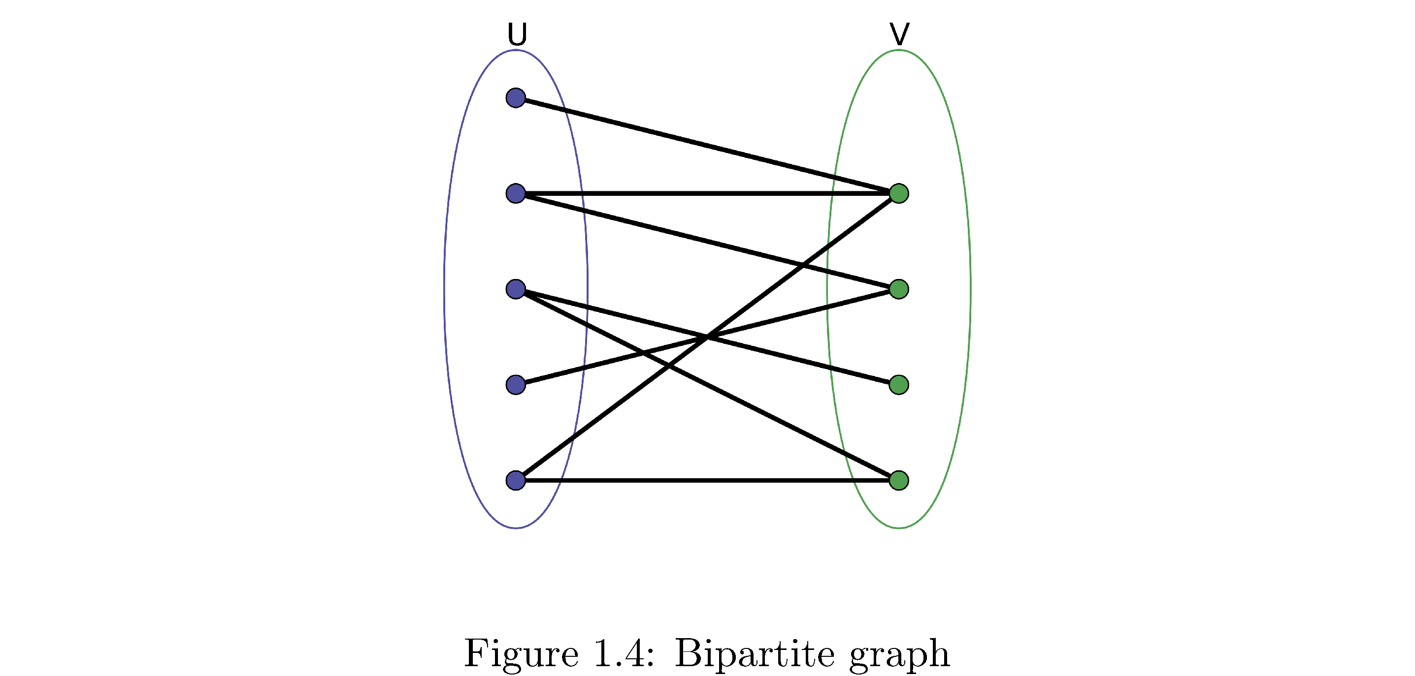
Graphs with particular properties get fancy names. A complete graph is a graph where every vertex has an edge to every other vertex (how many edges is that?). Figure 3 shows complete graphs for³ \(\left|V\right|=2,\dots,7\), i.e. 2 vertices, 3 vertices, …, 7 vertices. Are these unique? I.e is every other complete graph with \(7\) vertices isomorphic to \(K_{7}\)? A bipartite graph is a graph that can be divided into two sets \(V_{1},V_{2}\) such that the edges of the graph only connect vertices in \(V_{1}\) to \(V_{2}\) and vice versa (i.e. vertices in \(V_{1}\) are not connected to each other).

A bipartite graph is a graph that can be divided into two sets \(V_{1},V_{2}\) such that the edges of the graph only connected vertices in \(V_{1}\) to \(V_{2}\) and vice versa (i.e. vertices in \(V_{1}\) are not connected to each other). Figure 4 is a bipartite graph.

An acyclic undirected graph is a forest (need not be connected) and a connected, acyclic, undirected graph is a tree⁴. A directed acyclic graph is usually shortened to dag.

Finally the contraction of an undirected graph by an edge \(\left(u,v\right)\) is formed by removing the edge and making \(u=v\), i.e. contract \(u\) and \(v\) to be one vertex, with the edges connected to each of \(u,v\) now connected to the contracted vertex.

A weighted graph is one where the edges have numbers associated with them called “weights”. For example if vertices were cities in Florida and edges represented “being connected to by freeway” (any number of freeways but only freeways) then the edge weights might represent the number of highway changes you have to make when going from one city to another.

Representations of graphs

A representation of a graph is a data structure of some sort that captures information about the vertices and the edges connecting the vertices. The two standard representations are an adjacency list (which uses a list of linked lists) and an adjacency matrix (which uses a matrix obviously).

How to construct the adjacency list representation: first enumerate all the vertices of the graph (i.e. give each vertex a unique numerical “name”), then create a list or array type data structure of length \(n\) and for each entry in this list store another list. The index of the first list corresponds to some vertex and the list fetched upon indexing corresponds to all of the vertices its connected to. For example consider the graph in figure 5. The structure on the right is the adjacency list: the first column is an array or vector or something with pointers to the heads of linked lists. For example the 3rd position in the array corresponds to vertex 3 and hence has a pointer to a linked list that contains nodes (linked list nodes not graph nodes) that store the number identifying vertices that vertex 3 is connected to (a node with the number 6 and a pointer to another node with the number 5 [and the null pointer because vertex 3 isn’t connected to any other vertices]). Note that the order of the vertices as they appear in the linked lists don’t mean anything (for example 2 precedes 4 in vertex 1’s linked list but vertex 6 precedes vertex 5 in vertex 3’s linked list). Also note that since this is a directed graph the adjacency lists respect this: vertex 2 doesn’t have vertex 1 in its adjacency list.

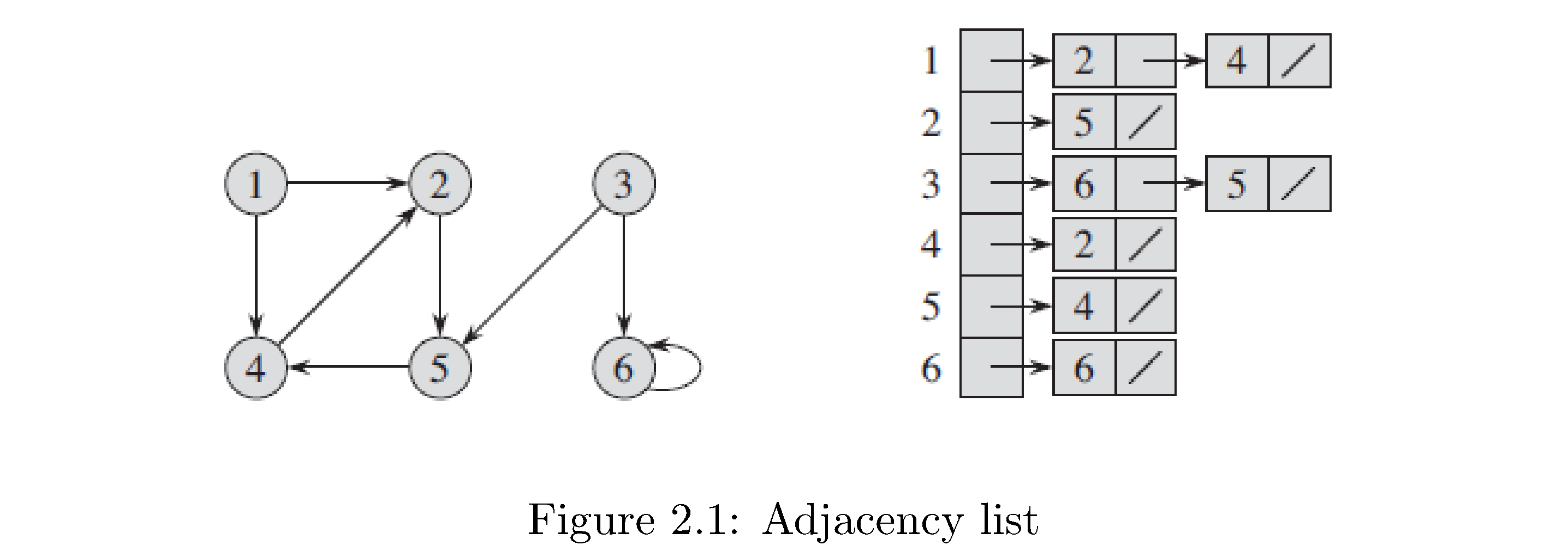
How to construct adjacency matrix representation: create a 2d array (matrix) of size \(\left|V\right|^{2}\) filled with zeros. Then fill in 1s on row \(i\) position \(j\) if vertex \(i\) is connected to \(j\). Figure 6 is the adjacency matrix representation for the graph in figure 5. Note that since this graph is directed the adjacency matrix representation respects this: just like for the adjacency list representation row 2 (corresponding to vertex 2) doesn’t have a 1 in the first position because there’s no edge from vertex 2 to vertex 1, but there is a 1 in the first row’s (the row corresponding to vertex 1) second position because there is an edge from vertex 1 to vertex 2. What would the graph look like if the graph was undirected? Hint: an undirected graph is like a directed graph but for any directed edge \(\left(i,j\right)\) there also exists directed edge \(\left(j,i\right)\).

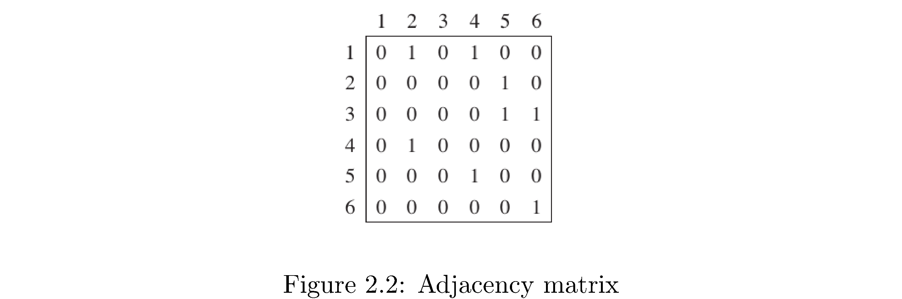
When is an adjacency list representation better than an adjacency graph representation? When the graph is “sparse”, which means vertices are on average adjacent to a small percentage of the other vertices. Why? Because adjacency lists store only information about present edges while the adjacency matrix explicitly stores zeros to indicate when 2 vertices aren’t adjacent. Notice that the matrix in figure 6 has many more numbers in it (if you count the zeros) than the adjacency list in figure 5. Conversely when a graph is “dense”, which means vertices are on average connected to a large percentage of the other vertices, the adjacency matrix representation is better because the added cost of traversing a linked list isn’t worthwhile for example if you’re trying to figure out if two vertices are adjacent (in the adjacency matrix representation you would just index directly to the other vertex and check for a 0 or 1 whereas in the adjacency list you have to traverse the list). For the adjacency list the space cost⁵ is \(\Theta\left(\left|V\right|+\left|E\right|\right)\) which means you need space proportional to the number of vertices (the length of the “top” array) and the number of edges (one linked list node for each edge). For the adjacency matrix representation the space cost is \(\Theta\left(\left|V\right|^{2}\right)\) regardless of the density or sparseness of the graph. Notice that if \(\left|E\right|=\left|V\right|\left(\left|V\right|-1\right)\), the maximum number of edges, then

\[\Theta\left(\left|V\right|+\left|E\right|\right)=\Theta\left(\left|V\right|+\left|V\right|\left(\left|V\right|-1\right)\right)=\Theta\left(\left|V\right|^{2}\right)\]

So worst case the space cost of an adjacency list representation is the same as that of the adjacency matrix representation.

Both representation can be adapted to represent weighted graphs. The linked list nodes in the adjacency list can be pointers to some other data structure that has fields that store weight attributes and the adjacency 2d array can similarly store pointers or simply have binary entries (the entries can be real numbers but note that in that case 0 weight might be semantically distinct from “not adjacent to” in which the case appropriate thing might be something like some entry representing \(\infty\)).

Breadth-first search

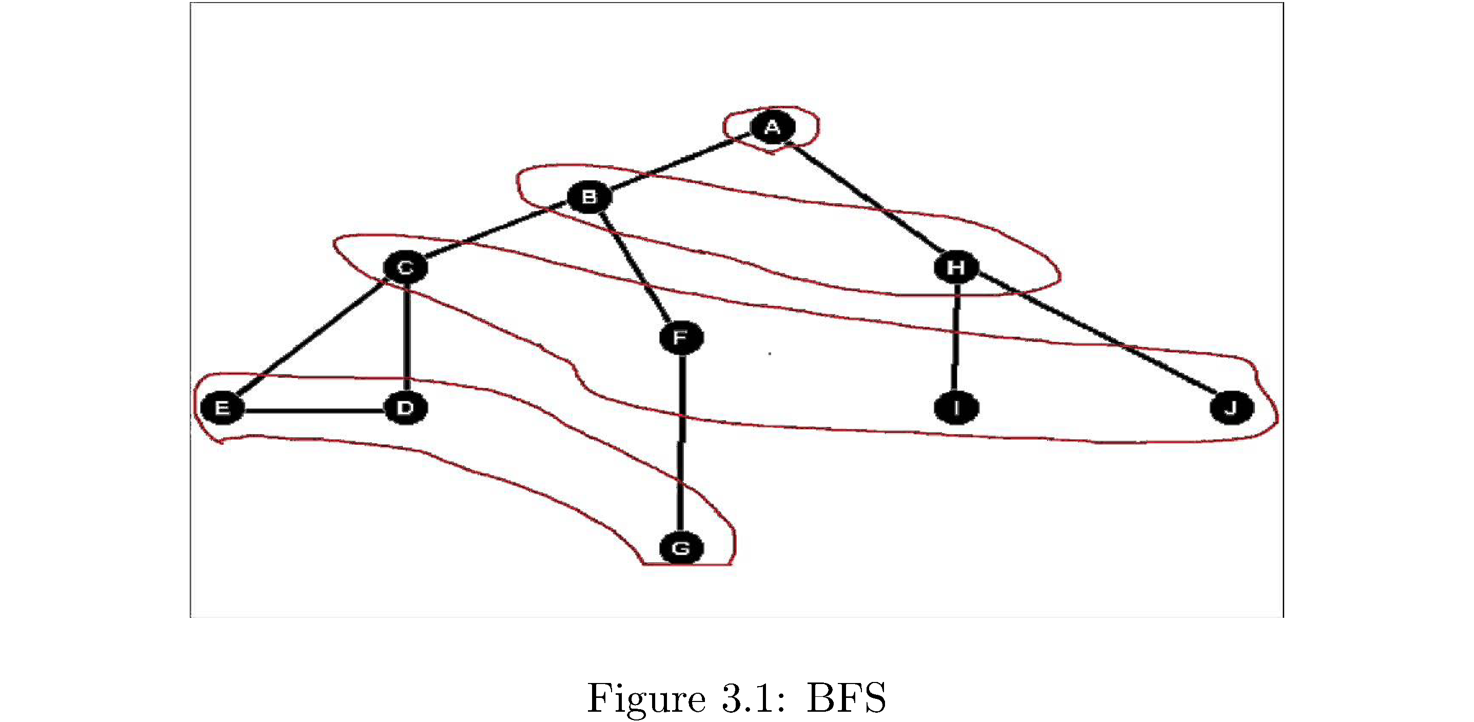
Breadth-first search (BFS) is better called breadth-first discovery because you’re not necessarily searching for anything you’re just exploring the graph. It’s the simplest thing you could think of doing: if you’re at some vertex “discover” all of its adjacent vertices then for each one of those discover each of its adjacent vertices, and so on. Note you go in order of discovery. So first discover all neighboring vertices \(v_{1},v_{2},\dots,v_{k}\) of some source vertex \(s\), then discover all the neighboring vertices \(v_{1,1},v_{1,2},\dots,v_{1,k'}\) of \(v_{1}\) and then move on to discovering all adjacent vertices of \(v_{2}\), not all adjacent vertices \(v_{1,1}\). So the discovery process goes in frontiers of number of edges from the source: discover all vertices within one edge of \(s\), then within two edges of \(s\), etc. Consider figure 7: The source is A from which B,H are discovered. From B the vertices C,F are discovered and then from H the vertices I,J are discovered. The levels are circled in red and correspond to frontiers of discovery.

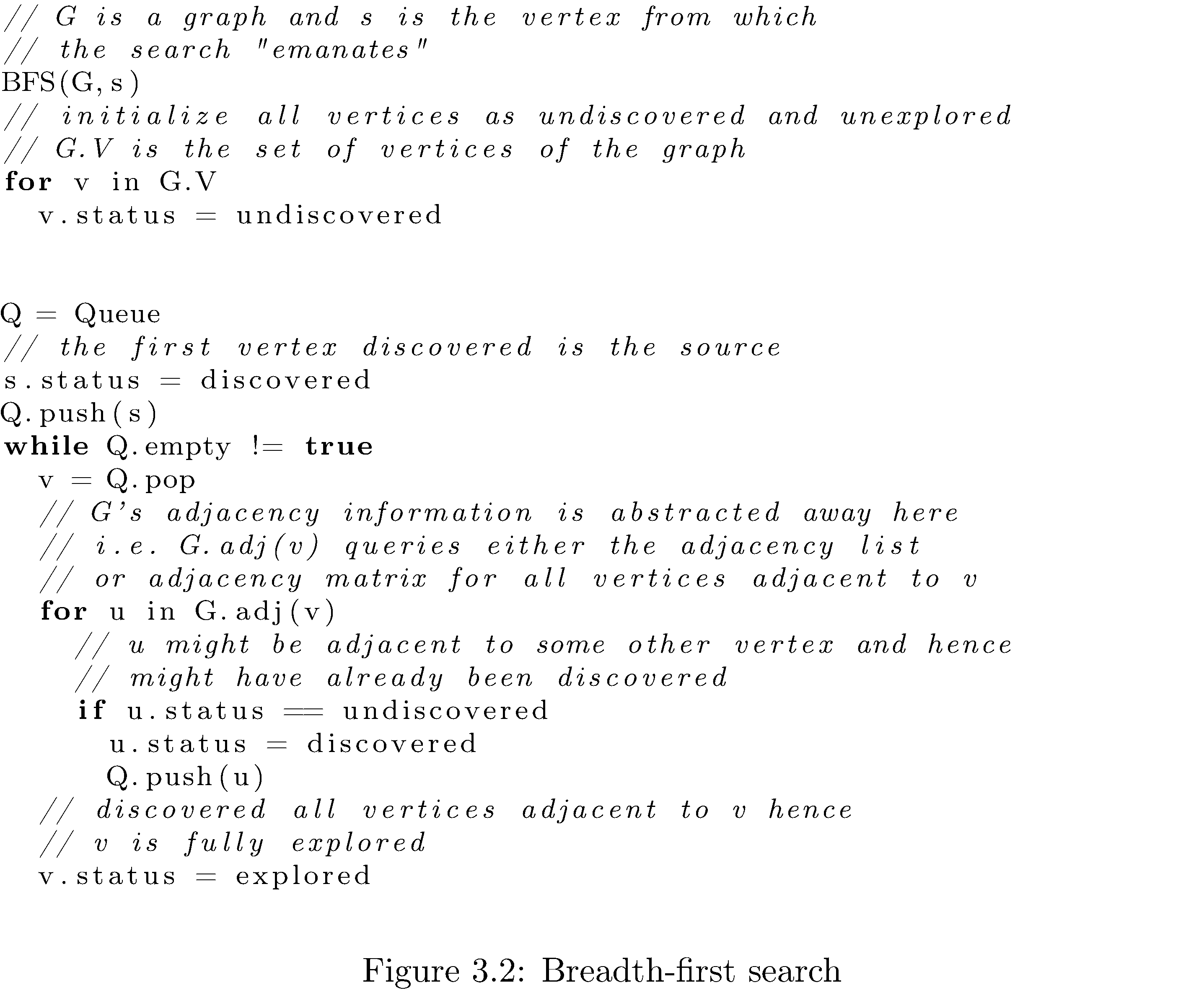
The order of visiting the vertices in BFS suggests an implementation: you want to discover the first vertex that’s one edge away, then the second vertex that’s one edge away, etc. until there are no more vertices one edge away. Then you want to “visit” the first vertex discovered at the one edge frontier and discover its “children”, then move on to the second vertex discovered at the one edge frontier and discover its “children” and so on. Hence you want to do the discovery process in a first in first out order: the vertices discovered earlier should be visited earlier. Obviously this suggests using a queue data structure. It’s also important to distinguish between vertices that have been discovered and those which have been fully explored so that vertices that have been discovered don’t get “re-discovered” (since a vertex might have an incoming edge from two other vertices in a preceding frontier) and those which have been fully explored don’t get explored again. Algorithm 8 lists pseudocode for a function that takes a graph \(G\) and a source \(s\) (from which to start the BFS) and performs the breadth-first search

That’s it - that’s basic BFS. What’s the runtime of BFS? Since you have to traverse each edge it’s \(O\left(\left|E\right|\right)\).

Now there are variations on the theme: for example you could use BFS to compute the number of edges from the source to every other vertex it’s connected to. How? Note that every vertex is one frontier deeper than the vertex “through which” it was discovered: so if the number of edges \(s.d\) from the source to itself is 0 then the number of edges from the source to each of the vertices discovered after exploring the source is \(s.d+1\). Setting this “distance” upon discovering the vertices adjacent to some vertex gives the correct distance of the discovered vertex from the source. Why? Because no vertex is discovered twice and so when \(u.d\) is set it’s set as early as it can be. There is also the notion of a breadth-first predecessor tree. This is basically a representation of which vertices were discovered by exploring which vertices in a breadth-first search. You can imagine rearranging the graph such that \(s\) at the center and the frontiers of vertices form concentric circles around \(s\). Figure 9 demonstrates this.

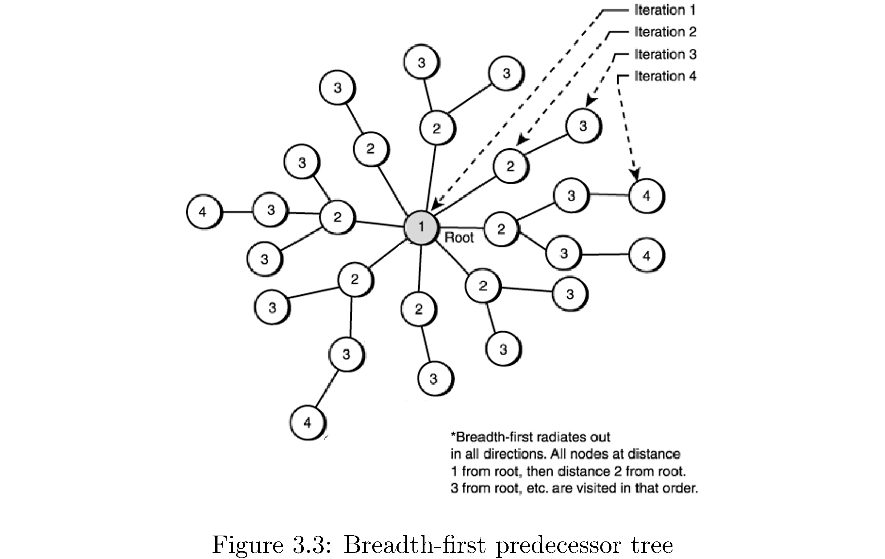
Formally for a graph \(G=\left(V,E\right)\) and \(s\) the breadth-first predecessor tree \(G'\) consists of all vertices \(V'\subset V\) that were discovered in a BFS emanating from \(s\) and edges \(\left(u,v\right)\in E'\subset E\) if \(v\) was discovered through exploring \(u\). It’s called a tree because there are no cycles (why?), it’s connected (why?). The “root” of the tree (figure 9) will be the source vertex \(s\). How would you construct the tree? Just keep track of which vertex a vertex was discovered through by storing a “parent” pointer that’s set when the vertex is discovered. Using the BFS predecessor tree you can also print out shortest paths to the source, in the sense of fewest edges, by following the parent pointers back to the source.

Dijkstra’s Shortest Path (Optional)

You haven’t read the section on depth-first search, nor topological sort, nor strongly connected components, but this section apperas here because topological sort and strongly connected components are applications of depth-first search and Dijkstra’s shortest path algorithm is an application of bread-first search.

As alluded to at the end of the BFS section you can use BFS to compute shortest paths from a single source to all vertices using a BFS tree. One way to think about the problem that that solves is computing the shortest path from a single source to all vertices on a weighted graph where all the edges have weight 1. But what if the edge weights aren’t one? It won’t work. BFS only gives you shortest path in the sense of fewest number of edges, not in terms of sum of edge weights (obviously since the algorithm never checks the edge weights). How could you use BFS to solve the problem of single source all vertices⁶ in terms of sum of all edge weights? Well if the edge weights are integral (have whole number values) one hack would be to insert \(k-1\) vertices on any edge with weight \(k\) and then the number of edges distance matches the edge weight distance. But that would blow up the run time of BFS since it’s \(O\left(\left|E\right|\right)\) and \(\left|E\right|\) will blow up.

The smarter way is to make BFS a little smarter: expand the frontier in the direction of the “nearest” vertices, where nearest now means those for which the path is shortest in the sense of sum of edge weights. In addition to expanding in the direction of the nearest vertices you should always update your current assessments of shortest paths to all vertices seen so far. Effecting the first part is easy: just replace the Queue in BFS with a Min-Heap where the priority ranking of each vertex its current shortest path distance from the source. Then the nearest vertices will be popped. To effect the second part is easy too: after popping a vertex update all of the distances to all of its neighbors if the shortest path to them (from the source) is shorter through the vertex that just got popped. The code appears in Algorithm 10.

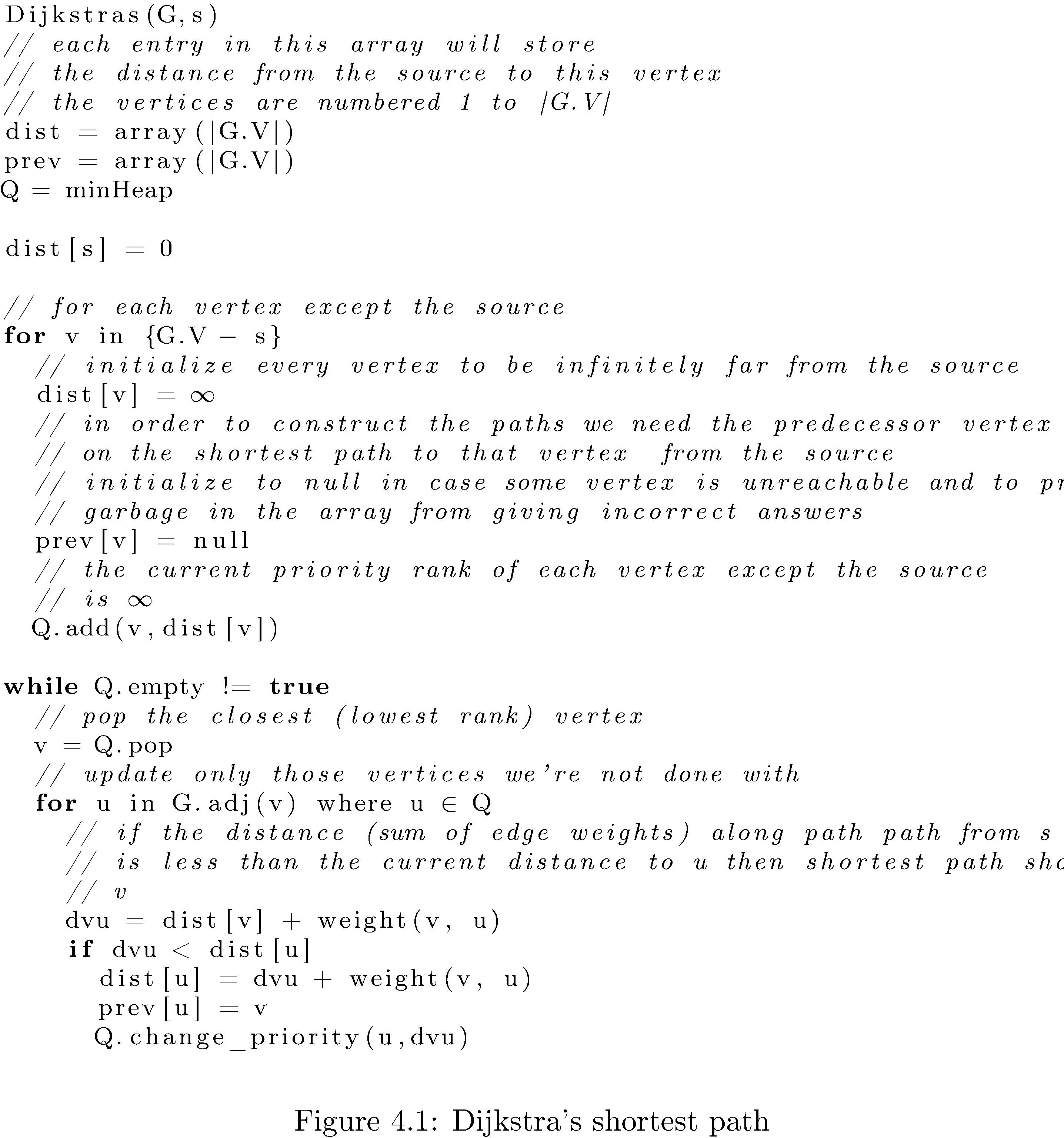
What’s the runtime of Dijkstra’s shortest path algorithm? The breadth-first search costs \(O\left(\left|E\right|\right)\) but since you have to do \(\left|V\right|\) insertions in the MinHeap, which each cost at most⁷ \(\log\left(\left|V\right|\right)\) (for example when the heap is almost full) the total runtime is \(O\left(\left|E\right|+\left|V\right|\log\left(\left|V\right|\right)\right)\).

Depth-first search

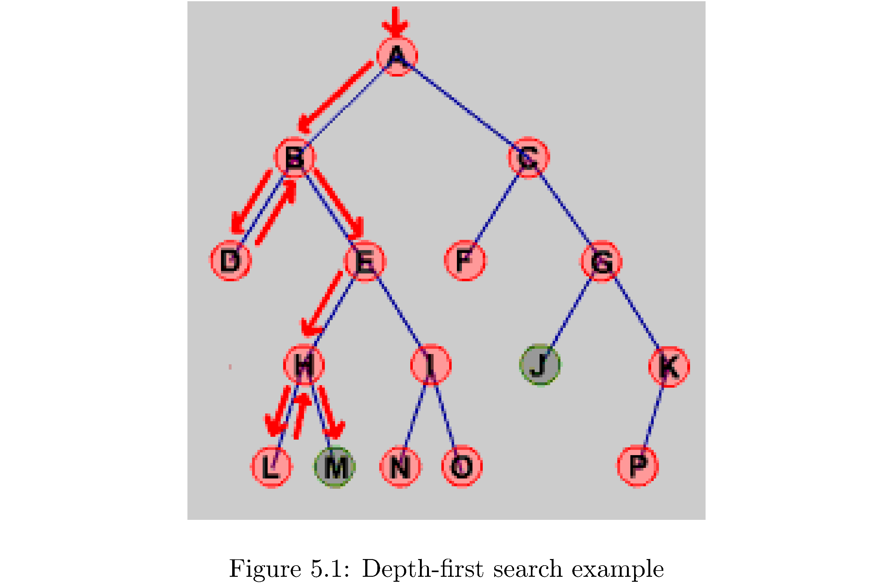
Depth-first search is almost exactly like breadth-first search except that it explores as deeply as possible (as opposed to as broadly as possible) on each iteration. Practically speaking the only difference is the replacement of the Queue with a Stack. Algorithm 12 shows the algorithm. Why should it be a Stack? The easiest way to see it intuitively is to go through an example on a small graph. Consider figure 11: first A is pushed (so it’s at the top of the stack), then popped and explored, then C and B are pushed (so B is at the top of the stack), then B is popped and explored, then E and D are pushed (so D is at the top of the stack, followed by E). D has no neighbors so E is the next to be popped and explored, pushing I and then H. The current state of the stack from bottom to top is (C,I,H). You get the idea. Essentially the Stack orders which vertices are to be explored by which were explored most recently (they appear at the top of the Stack!).

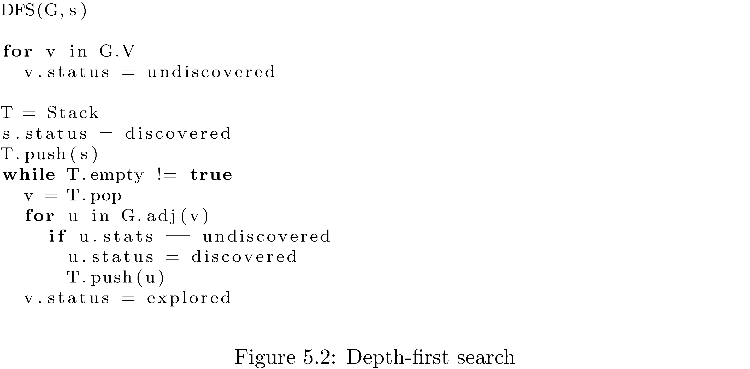
What’s the runtime of the algorithm? Since you need to traverse each edge in the worst case it’s \(O\left(\left|E\right|\right)\). Finally just like for breadth-first search you can construct a depth-first predecessor tree by keeping pointers.

Tangent: parentheses

The standard DFS algorithm can be easily modified to make it infinitely more useful: let’s keep track of when a vertex is first discovered, its “open” time, and when all of its children are done being explored, i.e. when it is “closed”. To enable this bookkeeping some trivial modifications need to made. Algorithm 13 is the modified algorithm.

How does the modified algorithm work? Keeping track of open times is easy: just keep a global timer (which you increment constantly) and assign the value of the timer to each vertex when it is discovered. The more difficult task is keeping track of the close time. Before even attempting to figure out what times to assign as close times note that in the unmodified algorithm the vertex is popped and disappears (in the sense that we don’t keep track of it anymore) so we couldn’t assign a time to it (whatever time) even if we wanted to. The solution is to “save” the vertex, i.e. don’t pop it. Hence peaking at it instead of outright popping it.

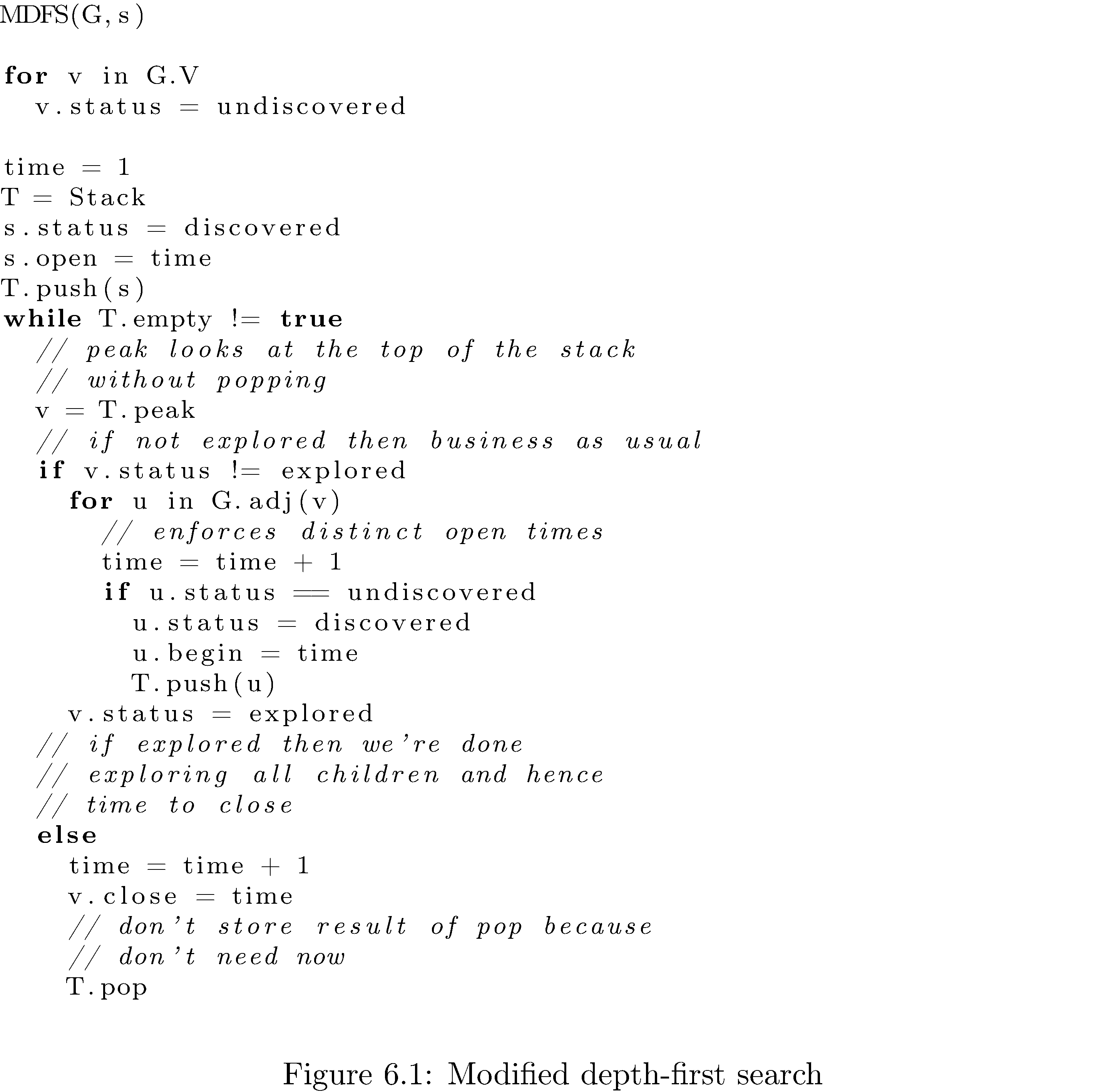
But now we need to distinguish between vertices on the stack because they are yet to be explored and those we’re saving just in order to assign close times to; hence the conditional. If the top of the stack is a vertex that hasn’t been explored then we do the same thing as the unmodified algorithm and if it’s one that has been explored then we know it’s one of those that we’re holding onto in order to assign it a close time. Also (coincidentally enough) if the top of stack is a vertex we’ve already explored that means that all of its children have been explored too (that’s the only way you “come back” to a vertex) and it should be closed. Note the counter is always incremented so that every open and close time is unique (i.e. no set of vertices has the same open time for example; it’s not possible for two vertices to have the same close time since the algorithm isn’t parallel).

What’s the use of all of this bookkeeping? We can the open and close times to “parenthesize” the vertices:

Theorem (Parenthesis): Given a DFS of a graph \(G=\left(V,E\right)\) for any two \(u,v\in V\) either the intervals \(\left[u.open,u.close\right]\) and \(\left[v.open,v.close\right]\) are entirely disjoint, i.e. \(u.close<v.open\) or one of \(\left[u.open,u.close\right],\left[v.open,v.close\right]\) is entirely contained in the other, i.e. \(u.open<v.open<v.close<u.close\).

What this theorem says is that for any two vertices \(u,v\) either they’re completely unrelated (e.g. \(u\) opens and closes before \(v\) opens and closes) or one of \(u,v\) is a ancestor of the other (e.g. \(v\) is “down the graph” from \(u\) and hence \(u\) opens, sometime later \(v\) opens, then eventually \(v\) closes, and sometime later \(u\) closes). Note this is not just about direct descendents, i.e. parents and children, but applies to any depth of descendance. Why is this called the parenthesis theorem? Look at this sequence of parentheses

\[\left(\left(\right)\left(\right)\left(\mathbf{\boldsymbol{(}\boldsymbol{)}}\left(\mathbf{\boldsymbol{(}}\left(\left(\right)\left(\right)\right)\mathbf{\boldsymbol{)}}\right)\right)\right)\]

and notice how for any two sets of parenthesesare disjoint (for example the bolded ones) or one is nested in the other.

In a sort-of but not completely related interesting tidbit if you wanted to test whether a set of parentheses was parenthesized correctly, i.e. nothing like )(()(, you’d use a stack. Can you think up how?

Topological Sort

A topological sort of a directed graph is a sorting of the vertices by precedence (i.e. which vertices “globally” precede which). For example figure \(\ref{fig:Topological-sort-of}\) is a topological sort of the graph in figure 1 that represents an order in which you can successfully get dressed: first socks, then undershorts, then pants, then shoes, then watch, etc. Note the edges are just reproduced from the graph - the topological sort is the order of vertices from left to right. I say an order because for example undershorts could be put on before socks because there’s no precedence relationship (no edge or sequence of edges) between socks and undershorts. Another name for a topological sort is a linearization of a graph (because it kind of arranges the vertices in a line).

A topological sort only makes sense for a directed graph - there is no notion of precedence in an undirected graph. Furthermore a topological sort is only possible in a directed acyclic graph. Why? If there’s a cycle in the graph then which vertex in the cycle really precedes which other vertex? The precedence of the vertices in the cycle with respect to each other is ill-defined. How do you detect a cycle in a directed graph? Easy: if at some point during a depth-first search you were about to “discover” a vertex that had already been discovered (i.e. but not explored) then there’s a cycle. Why? Since all discovered vertices get turned into explored vertices as the DFS “comes back up” the only way to see a discovered vertex that hasn’t been fully explored is if the DFS has looped back. Therefore assume without loss of generality that the directed graphs in this are directed acyclic graphs (meaning before you try to do a topological sort of a graph check to see if it’s acyclic).

How do you do a topological sort of an acyclic graph? Easily! Do a depth-first search and just list the vertices in reverse order of their closing times. I’ll repeat that again: list the vertices in reverse order of their closing times not their opening times!!! Why? As a warm-up think about it like this: what is the closing time of ‘undershorts‘ in figure 1 if I start the depth-first search at it? It’ll be one of the last ones⁸ because everything below it will close before it (since everything below it is a descendent of it and by the parenthesis theorem). Now figure 1 is kind of strange because ‘socks‘ is never discovered by a depth-first search starting at ‘undershorts‘. The solution is essentially to rerun depth-first search start at vertices that remain undiscovered while keeping the timer global. The algorithm appears in Algorithm 15.

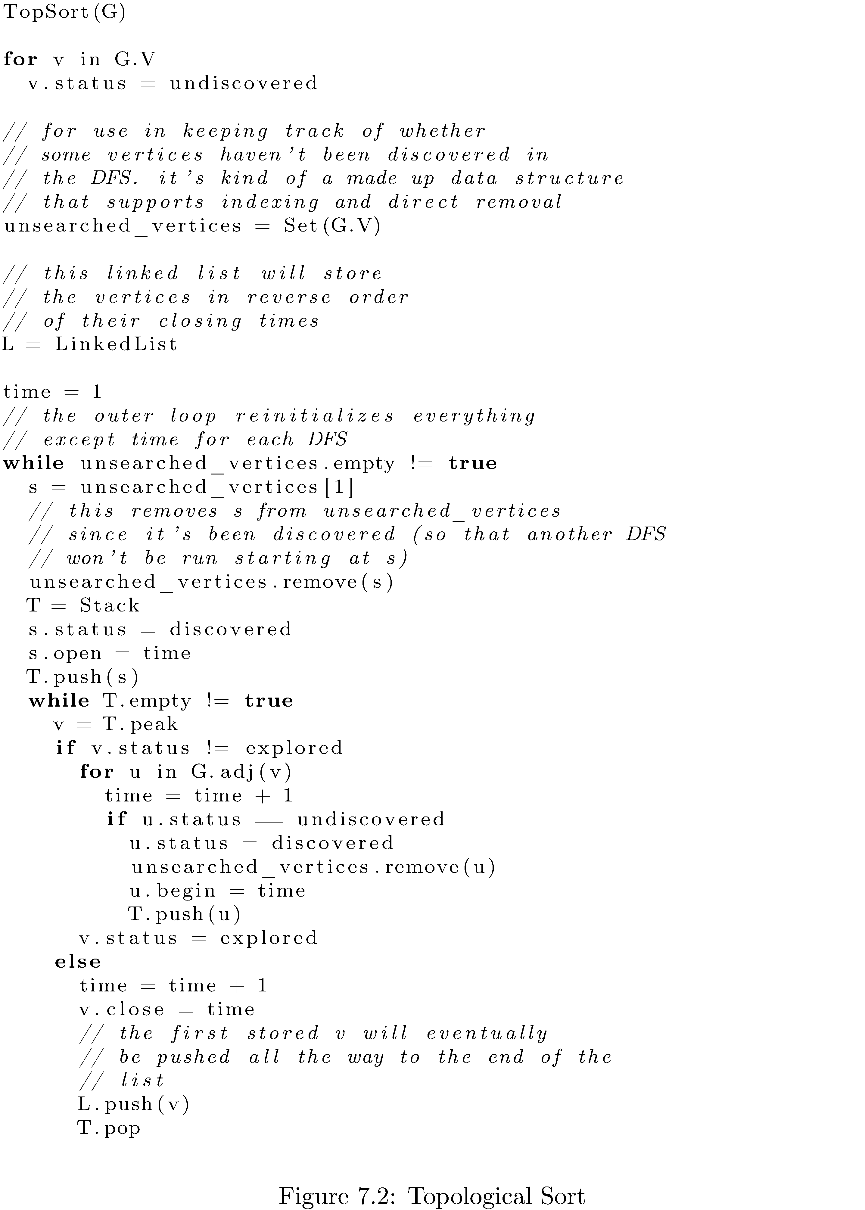
What’s the runtime? Since it’s essentially a DFS the runtime is \(O\left(\left|E\right|\right)\).

Strongly Connected Components

Recall that a connected component of a undirected graph \(G\) is a subgraph \(G'\) that’s connected, i.e. each vertex can reach each other vertex. A strongly connected component is the same thing in a directed graph. A graph could have many distinct (unreachable from each other) connected components. How would you find them all? For an undirected graph it’s easy: use either breadth-first search or depth-first search. Since the graph is undirected any path from a vertex \(u\) to a vertex \(v\) can be similarly used by \(v\) to reach \(u\). For directed graphs it’s a little more difficult…

How about an intuition pump⁹: consider the directed graph in figure 16

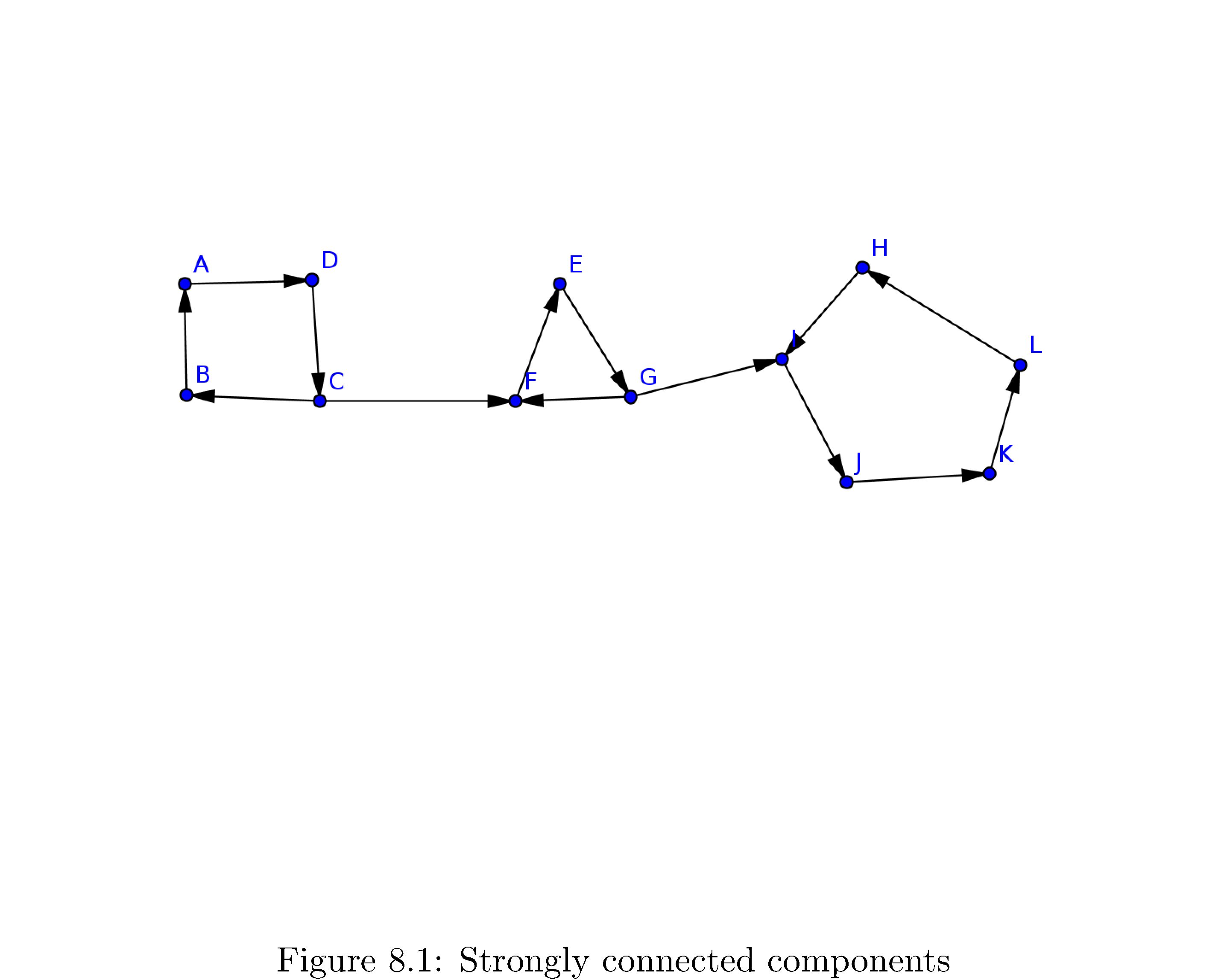
. First of all do you recognize the connected components? They are

\[\begin{align} C_{1} & =\left\{ A,B,C,D\right\} \\ C_{2} & =\left\{ E,F,G\right\} \\ C_{3} & =\left\{ H,I,J,K,L\right\} \end{align}\]

Note that the entire graph is not strongly connected (since, for example, \(A\) is unreachable from \(K\)).

So how would algorithmically decide all of the connected components in this graph? Maybe a first guess would be to perform a depth-first search from and see which vertices are discovered by that depth first search. That clearly doesn’t work because all vertices are reachable from \(A\). In contrast how about a performing a depth-first search that starts at \(H\)? Well then the only vertices discovered will be \(\left\{ H,I,J,K,L\right\}\). That’s \(C_{1}\) the connected component \(H\) is a member of! This is very close to what we need but this doesn’t work iforms a cycle. All of the vertices you can reach from some fixed vertex (e.g. \(F\)) are not all in that vertex’s strongly connected component. To drive the point home: if you had started the DFS at \(F\) you would have discovered

\[\left\{ E,F,G,H,I,J,K,L\right\} =C_{1}\cup C_{2}\]

Not all of the discovered vertices are in \(F\)’s connected component but all of vertices in \(F\)’s connected component are discovered!

What’s the key feature here? Look again at \(C_{3}\) and think about what happens when you perform the depth-first search starting at \(H\). The DFS discovers all the vertices in the “last” part of the graph only because it’s stuck; because the edge \(\left(G,I\right)\) only goes one direction the DFS can’t get out. This is the key. If you knew what the “last” part of the graph was you could run DFS on it, collect all the vertices discovered and label them as one strongly connected component, remove all of them, then rerun DFS on the “second to last” part, etc.

This is almost the answer but it’s not, unfortunately. Consider the graph in figure 17

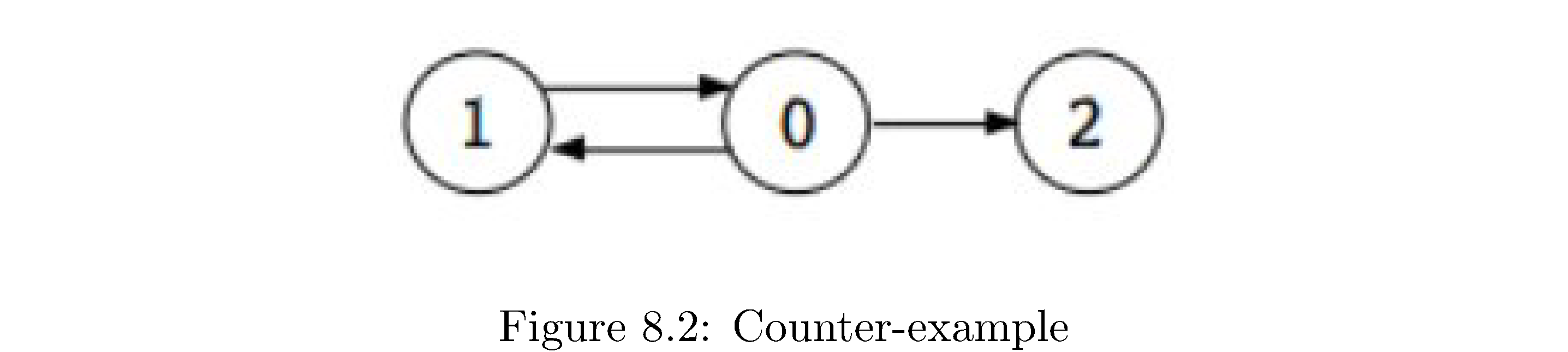
. A plausible DFS that starts at \(0\) gives finishing ordering of first 1, then 2, then 0. Then your second DFS, starting at 1, would produce \(\left\{ 1,0,2\right\}\) as a strongly connected component since both 0 and 2 are reachable from 1. The reason for this, vaguely, is that there’s no well defined “last” part of the graph. But there is a well defined “first” part to the graph (at least relative to where you start the DFS from)! A topological sort¹⁰ gives you the “first” part as the vertex with the highest finishing time. But how can we use this since the whole algorithm hinges on “getting stuck” and clearly for graphs like in figure 16 you wouldn’t get stuck if you started at \(A\).

The solution is to use, for the second depth-first search the transpose graph¹¹, i.e. flip all the edges in the original graph. Note that the strongly connected components of \(G^{T}\) and \(G\) are the same¹²so there’s no loss of reachable paths. So now you can effect the same idea (using the “getting stuck” nature of the second DFS) on the “first” part of the graph: just start the second DFS on the vertex with the highest finishing time (i.e. the one that’s topologically sorted to be the first in order). Once you identify the strongly connected component of the “first” part of the graph, remove all those vertices and do the same thing with the next highest finishing time vertex that’s still left. The source appears in Algorithm 18.

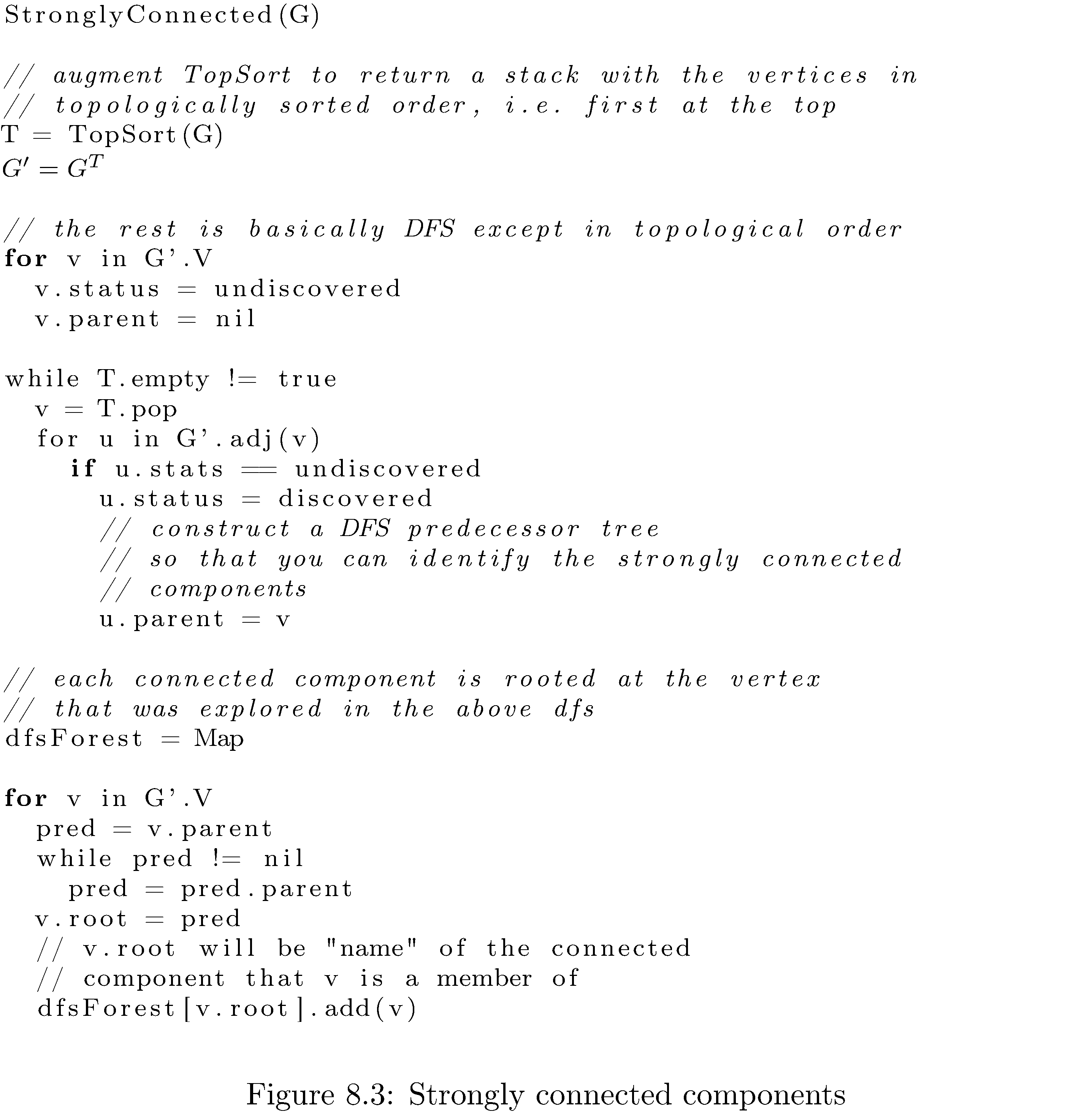
What’s the runtime of the algorithm? Each DFS takes \(O\left(\left|E\right|\right)\) but the computation of the transpose graph takes \(O\left(\left|V\right|+\left|E\right|\right)\) so the total runtime is \(O\left(\left|V\right|+\left|E\right|\right)\).

Footnotes